CME SOFR Futures and SOFR Volatility

CME One-Month SOFR futures can be used to evaluate and manage day-to-day volatility in Treasury general collateral repurchase agreement (GC repo) rates, particularly around month-end dates. In what follows, we examine a couple of recent episodes to show how.

SOFR

In mid-2017, the Alternative Reference Rates Committee (ARRC) endorsed SOFR (the Secured Overnight Financing Rate, published daily by the Federal Reserve Bank of New York (FRBNY) as “the rate that represents best practice for use in certain new USD derivatives and other financial contracts, representing the ARRC’s preferred alternative to USD LIBOR. SOFR is a broad measure of the cost of borrowing cash overnight collateralized by U.S. Treasury securities in the repurchase agreement market.”¹ “The repo market represents a liquid, efficient, tested and safe way for firms to participate in a short-term financing arrangement, providing funding for their day-to-day business operations.”²   In short, the GC repo market is the grease that keeps the wheels of the US government securities market turning.

SOFR began regular daily production in the first week of April 2018.

 

CME SOFR Futures and SOFR Volatility

A month later, CME Group launched two new futures products based on it. Each Three-Month SOFR (SR3) futures contract is based on daily compounded SOFR interest during the contract’s three-month reference period. Each One-Month SOFR (SR1) futures contract references the arithmetic average of daily SOFR values over all days in the contract month. Both futures products have multiple delivery-month listings.³

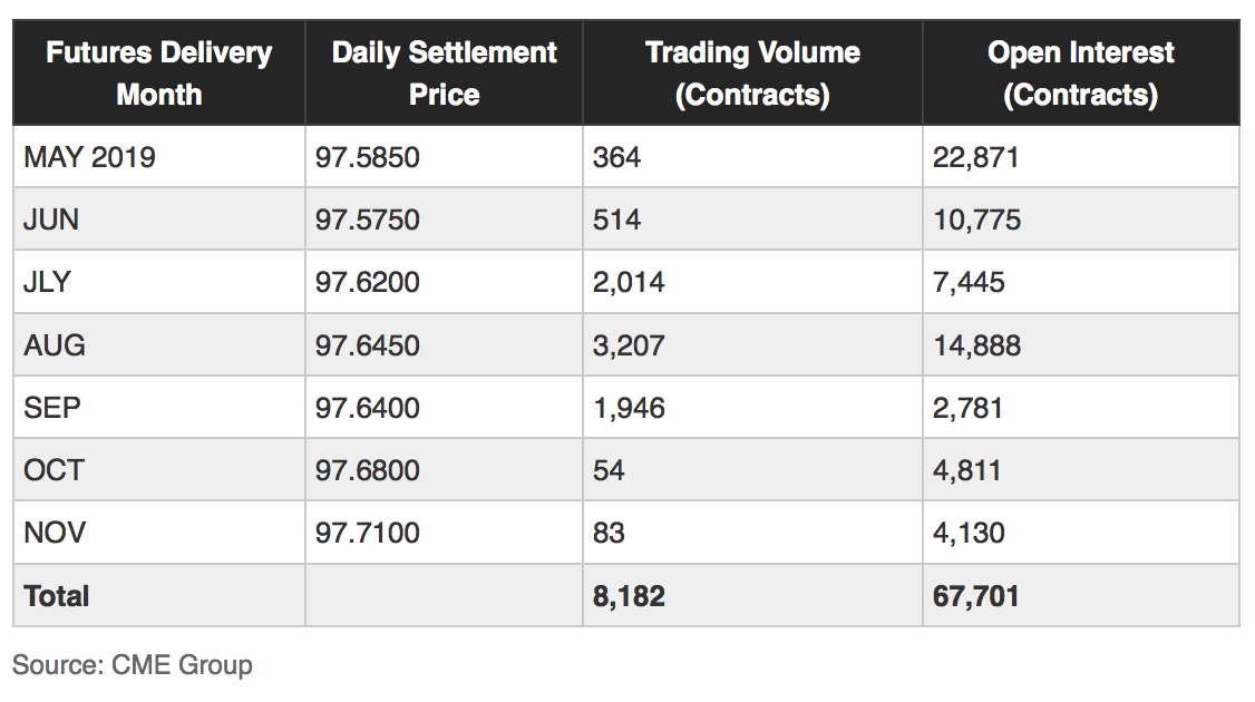
For SR1 futures, daily settlement prices, trading volumes, and open interest levels are exemplified by data for Friday, 10 May 2019, shown in Figure #1.

Figure 1 – CME SR1 Futures, Friday, 10 May 2019

In Figure 2, which depicts recent history of the daily effective federal funds rate (EFFR) and SOFR, two features are notable. One is the generally strong correlative relationship between the two benchmarks. The EFFR-minus-SOFR spread is centered on an average of -10 basis points (bps) per year.

Figure 2 – Daily EFFR and SOFR, May 2018-May 2019

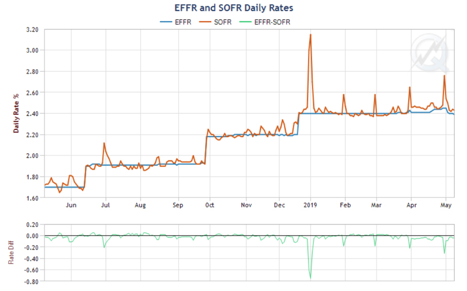
The other is the occurrence of transitory departures from the prevailing average, noticeably around month-end dates. Such events at year’s end, commonly known as “the turn”, are long-familiar to money market practitioners. At the close of 2018, for example, increased demand for collateralized cash balances drove SOFR to 76 basis points (bps) over EFFR. 

Both of the CME SOFR futures contract mechanisms absorb and reflect such events without difficulty. Their respective designs incorporate the principle (highlighted in the ARRC’s recently published “User’s Guide to SOFR”) that financial products based on overnight interest rate benchmarks do well to reference period-averages instead of single-day values:

“There are two essential reasons why financial products use an average of the overnight rate:

• First, an average of daily overnight rates will accurately reflect movements in interest rates over a given period. For example, SOFR futures and swaps contracts are constructed to allow users to hedge future interest rate movements over a fixed period, and an average of the daily overnight rates that occur over the period accomplishes this.
• Second, an average overnight rate smooths out idiosyncratic, day-to-day fluctuations in market rates, making it more appropriate for use.”⁴

Given this, how might SR1 futures be used either to manage calendar-related volatility in SOFR or to take a view on it?

Example 1 – November 2018

To answer by example, let’s start with November 2018, for which Figure #3 presents various data for each day:

• SOFR value,
• month-to-date arithmetic average of daily SOFR values (“Avg SOFR to Date”),
• trade-volume-weighted average (TWA) price of November 2018 SR1 (SR1X8) futures,
• expected average of daily SOFR values during the month, as implied by SR1X8’s TWA price,
• market expectation of the average daily SOFR level for the remaining days of the month, as implied jointly by SR1X8’s TWA price and daily SOFR values published from start of month through the preceding business day (“Implied Avg SOFR to Month End”), and
• SR1X8 trading volume.

Figure 3 – SOFR and SOFR Futures Rates, Prices, and Volumes, November 2018 (pct/yr, unless otherwise indicated)

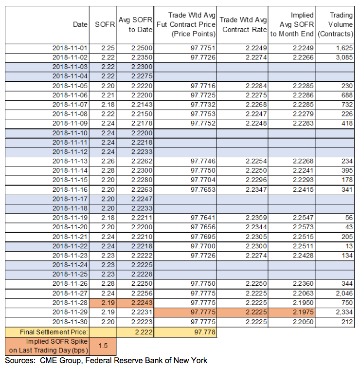
The futures contract final settlement price, shown in the next to last row, is 100 price points minus the arithmetic average of daily SOFR values during the month:  100 – 2.222 = 97.778. (In accord with the product rules, the SOFR value assigned to any weekend day or holiday is the value corresponding to the first preceding US government securities market business day, and the month-average value is rounded to three decimal places – the nearest 1/10^th of one basis point (bp) per annum of SOFR interest – before being subtracted from 100.)

Figure 3 illustrates how the averaging process that informs the final settlement price smooths out daily SOFR values (eg, the intramonth high of 2.28 pct on 14 November, or the intramonth low of 2.18 pct on 19 November).

Figure 3 also suggests how SR1 futures users might use contract price information to gauge market expectations as to the magnitude of month-end SOFR volatility. To see this, suppose it is Thursday, 29 November, the next-to-last day of trading in the contract.

• FRBNY already has published SOFR values for each of the preceding 28 days of the month. Average SOFR for those 28 days is 2.2243 pct/yr (highlighted in red).
• The transaction-weighted average futures price during the 29 November trading session is 97.7775, implying that market participants collectively look for the average SOFR level during the month to be 2.2225 pct/yr, equal to 100 minus 97.7775 (both highlighted in red).
• In turn, these two results jointly imply a market consensus expectation that the average SOFR level for the remaining two days of the month (Thursday, 29 November, and Friday, 30 November) is:
  
  2.1975   pct/yr  =   [ (30 days x 2.2225 pct/yr) minus (28 days x 2.2243 pct/yr) ] / (2 days)

What might this imply for market expectations of SOFR’s behavior at month’s end?  One of potentially many ways we could answer is to impose two side assumptions:  First, in the absence of any calendar-related divergence, SOFR will hold steady at its latest published value of 2.19 pct/yr (highlighted in red) on each of the remaining two business days of the month; second, any calendar-related divergence will occur entirely on the last business day of the month.

With these two side assumptions, the result could be interpreted to indicate that market expectations are centered on SOFR values of:

• 2.19 pct/yr for Thursday, 29 November, and
• 2.205 pct/yr⁵, equal to a baseline value of 2.19 pct/yr plus a month-end premium of 1.5 bps/yr, for Friday, 30 November.⁶

With the data available to us and with a couple plausible assumptions, we can venture a reasonable guess that market participants collectively foresee month-end calendar effects pushing SOFR 1.5 bps higher than it would be otherwise.

In the event, this prediction would have proven tolerably good. The published value of SOFR for Thursday, 29 November, was 2.19 pct/yr, as assumed. For Friday, 30 November, it was 2.20 pct/yr instead of 2.21 pct/yr.

Two features of the outcome merit remark –

1. The magnitude of month-end calendar-related distortion in SOFR – both predicted and actual – was so small in this case as to be imperceptible. Lately, daily SOFR values vacillate half the time within a range of 2 bps above or below their local median level. Given this, a month-end bump of +1.5 bps would have passed without notice.
2. Given the calendar configuration of November 2018, and given the SR1 product rules governing assignment of daily SOFR values to weekend days and US government securities market holidays, the value on the last day of the month — no matter how large or small — was destined to be limited in impact to 1/30^th of the month-average level.

Example 2 – March 2019

For contrast, consider an alternative scenario:

• in which higher month-end volatility in SOFR might reasonably be anticipated (owing to quarter-end corporate balance-sheet reporting pressures, for instance), and
• for which the potential impact of month-end volatility in daily SOFR upon the month-average SOFR level is greater, because the SOFR value for the last business day of the month counts for multiple days instead of just one.

The March 2019 delivery month (SR1H9) makes an ideal specimen. As Figure 4 evidences, its last day is a Sunday, which means that the SOFR value for the last business day of the month, Friday, 29 March, exerts impact upon nearly 1/10^th of the month-average value (three days out of 31) that determines the final settlement price.

To appreciate the implications, assume as before that it’s the contract’s next-to-last trading day, Thursday, 28 March.

• The average of published SOFR values for the first 27 days of the month is 2.4052 pct/yr (highlighted in red).
• The transaction-weighted average futures price during the 28 March trading session is 97.5308, indicating that market participants’ collective expectation is for the month-average SOFR level to emerge around 2.4692 pct/yr (equal to 100 minus 97.5308).
• By implication, the market consensus expectation is that the average SOFR level for the remaining four days of the month will be:
  
  2.8854   pct/yr  =   [ (31 days x 2.4692 pct/yr) minus (27 days x 2.4052 pct/yr) ] / (4 days)

Likewise, suppose we apply simplifying assumptions similar to the two we used earlier:  SOFR holds steady at its last published value, 2.40 pct/yr, on each of the remaining two business days of the month in the absence of any month-end calendar effects; and any calendar-related divergence occurs entirely on the last business day of the month, Friday, 29 March.

The forecast path that emerges places SOFR at:

• 2.40 pct/yr on Thursday, 28 March, and
• around 3.05 pct/yr on Friday, 29 March, comprising a baseline value of 2.40 pct/yr plus an estimated month-end jump of 64.7 bps.⁷
• Given the configuration of the calendar, and given the product rules, Friday’s SOFR value – whatever it turns out to be – is assigned to the ensuing Saturday and Sunday.

Figure 4 – SOFR and SOFR Futures Rates, Prices, and Volumes, March 2019 (pct/yr, unless otherwise indicated)

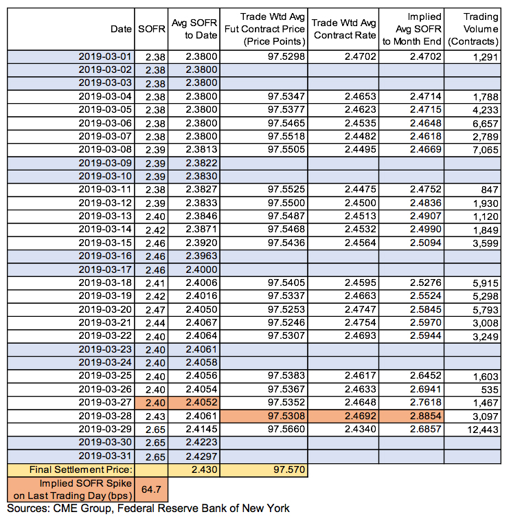
In fact, the month-end rise in SOFR turned out to be around 25 bps (equal to actual SOFR of 2.65 pct/yr minus the baseline prediction of 2.40 pct/yr). Although this is significant, it is modest relative to the 64.7 bps predicted according to the scheme described here.

The next day — contract’s last trading session, Friday, 29  March — is notable for at least two reasons:

• Trading volume, at more than 12,400 contracts, was heavy for an expiring contract, remarkably so for one that expires by reference to a lengthy period-average of daily benchmark values.
• Market participants made use of that trading session to refine their collective assessment of the size of the month-end effect. The trade-value-weighted average price for the day, 97.5660 price points, is consistent with a market consensus expectation that SOFR’s average level for the month would be 2.4340 pct/yr. Combined with published SOFR values for 1 March through 28 March, this implies that market participants collectively looked for SOFR to clock in at roughly 2.69 pct/yr on Friday. Given the magnitude of day’s volatility in Treasury GC repo rates, this lands remarkably close to the 2.65 pct/yr that FRBNY published the following Monday.

Risk Management

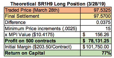
As Figure 5 illustrates, a hypothetical trader who acquired a long (short) position of 500 SR1H9 contracts at 97.5325 on 28 March, and who offset this position by holding it to final settlement, at the final settlement price of 97.570, would have realized a profit (loss) of 0.0375 price points, or $78,131.25.

Given that the initial margin requirement for SR1 futures at the time was $203.50 per contract, initial margin for this position would have been $101,750.

Figure 5 – Profit/Loss on Hypothetical Long Position in SR1H9, 28 March 2019

 

Summary

The examples here underscore the usefulness of the CME SOFR futures mechanism. By averaging SOFR across an entire contract month, it smooths day-to-day fluctuations in the underlying SOFR benchmark. Yet it preserves enough flexibility for hedgers and speculators to effectively manage risk arising from SOFR volatility. This is especially useful around month’s end, when overnight Treasury GC repo rates often become more challenging to predict.

 

References

1. Alternative Reference Rates Committee, “A User’s Guide to SOFR”, page 5, April 2019, https://www.newyorkfed.org/medialibrary/Microsites/arrc/files/2019/Users_Guide_to_SOFR.pdf

2. SIFMA, “US Repo Market Fact Sheet, 2018”, September 2018, available at:  https://www.sifma.org/resources/research/us-repo-market-fact-sheet-2018/

3. For more information, see contract specifications at:  /content/cmegroup/en/trading/interest-rates/stir/three-month-sofr_contract_specifications.html and /content/cmegroup/en/trading/interest-rates/stir/one-month-sofr_contract_specifications.html

4. Alternative Reference Rates Committee, “A User’s Guide to SOFR”, page 3, 22 April 2019, available at: https://www.newyorkfed.org/medialibrary/Microsites/arrc/files/2019/Users_Guide_to_SOFR.pdf

5. As a practical matter, SOFR would never take a value of 2.205 pct/yr, because FRBNY rounds each day’s SOFR value to two decimal places before (ie, to the nearest bp) before publishing it.  In this hypothetical example, if the computed value of the trade-value-weighted median of SOFR-eligible overnight Treasury GC repo rates on the last day of the month were exactly 2.2050 pct/yr, then FRBNY would round this to a published value of 2.21 pct/yr.

6. The arithmetic that provides the check is:  2.1975 pct/yr   =   (2.19 pct/yr   plus   2.205 pct/yr) / 2

7. The arithmetic to check the result is:  2.8854 pct/yr   =   [ (1 day x 2.40 pct/yr) plus (3 days x 3.047 pct/yr) ]  /  4 days

 

Stay informed on CME Group’s Interest Rate markets, providing the latest product updates, market trends, new research and tools, and more

Sponsored content