FVA – Time to go asymmetric?

Despite being introduced over six years ago, there is still no market consensus on how to calculate funding valuation adjustments – known as XVAs. One point of contention is whether to use the same funding curve for borrowing and lending (symmetric funding) or to use different curves to reflect the real bid/offer that banks incur in the market (asymmetric funding). Stuart Nield, XVA product manager at IHS Markit, reviews the difference between the two approaches, discussing the technical challenges involved and providing evidence for why banks should make the switch to asymmetric funding sooner rather than later

 

Funding valuation adjustments (FVA) calculation

FVA can be broken down into two components: the funding cost adjustment (FCA), arising when the derivatives business requires funding; and the funding benefit adjustment (FBA), arising when the derivatives business generates funding. These two components use banks’ lending and borrowing spreads respectively, as shown in figure 1 (where the survival probability has been omitted for simplicity).

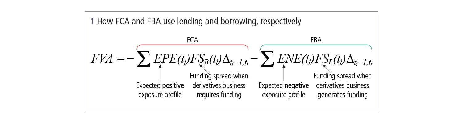
A key property of this formula is that it is performed across the entire derivatives portfolio – cash received for derivatives funding can be rehypothecated across all trades. The two funding spreads used for calculating FCA and FBA are typically set by the bank’s internal treasury.

 

Technical challenges

Determining the expected positive exposure (EPE) and expected negative exposure (ENE) across the entire derivatives portfolio calls for a global simulation of all the trades in a bank’s portfolio. This can prove difficult for legacy systems that were designed at the beginning of the XVA journey because the early valuation adjustments – credit value adjustment (CVA) and debit valuation adjustment – were built on counterparty-centric simulation workflow. The difference between the global simulation approach – which is required for asymmetric FVA – and the counterparty-centric simulation approach is illustrated in figure 2.

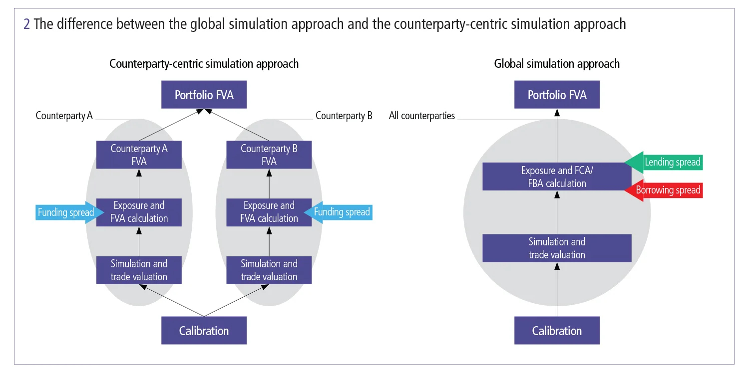
In a counterparty-centric simulation, each counterparty is treated separately – only risk factors in each counterparty’s portfolio are simulated. This technique keeps the simulated data relatively small because only the relevant assets are simulated, reducing memory requirements. However, this simplicity comes at a cost – the random numbers used across counterparties will be different, giving inconsistent scenarios across the entire portfolio. This means trade valuations on a per-path basis cannot be added across all derivatives – which is required to calculate asymmetric FVA.

In contrast, a global simulation simulates all risk factors in the derivatives portfolio simultaneously, giving scenario consistency across all trades. Trade mark-to-market matrices can be aggregated across the entire derivatives portfolio, allowing EPE and ENE to be calculated at the total portfolio level. Different curves can then be used to calculate FBA and FCA as in the equation presented in figure 1.

Institutions using counterparty-centric simulation are forced to use only symmetric funding in calculating FVA because the counterparty-level EPEs and ENEs cannot be added up to the portfolio level due to scenario inconsistency. Asymmetric FVA is beyond their reach.

 

Case study

To understand the impact of switching to asymmetric funding, IHS Markit configured an example portfolio using its Front-Office XVA Solution. This system is built using big data technologies and can therefore perform a global simulation, allowing users to calculate both symmetric and asymmetric FVA at the total portfolio level. The example portfolio contained:

• 70 counterparties with names seen in typical European XVA portfolios
• 1,000 foreign exchange and interest rate trades across four major currencies
• Products including interest rate swaps, cross-currency swaps, callable swaps and forex forwards.

 

Banks typically have asset-heavy portfolios (trades are deep in the money) because long-dated rate receiver and inflation swaps initiated in the early 2000s increased in value as rates dropped following the 2008 credit crisis. The example portfolio has been configured to reflect a typical bank and so it is asset heavy.

A key input to the FVA calculation is the level of the funding curve, which is not directly observable in the market. However, a typical funding level can be inferred from IHS Markit’s Totem XVA service. This curve is presented as the borrowing spread in figure 3.

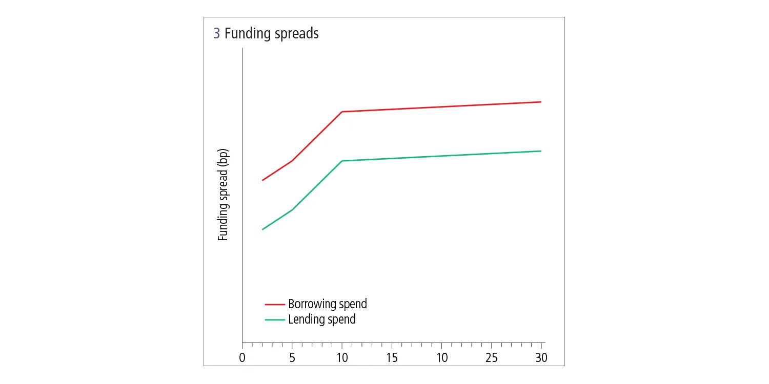
The lending spread curve was assumed to have a 20 basis point negative spread to the borrowing curve, as shown in figure 3.

Running the FVA calculation yields the following results for the total derivatives portfolio. For symmetric funding, the same curve has been used – the borrow curve – to compute FVA, but for asymmetric funding both curves were used (see figure 4). 

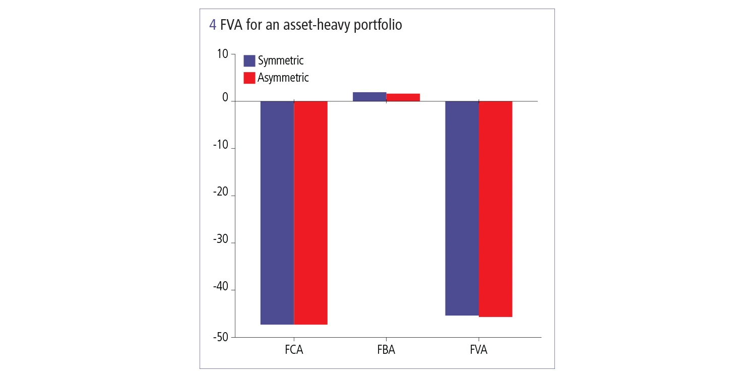
There is only around 1% difference between symmetric and asymmetric funding for the asset-heavy portfolio. This result stems from the fact the FCA, which uses the borrow spread, dominates over the FBA, which uses the lending spread – meaning its sum (the FVA) is mostly FCA.

But what happens as the portfolio becomes more balanced? This is an important question as banks have recently been making their derivatives portfolios more balanced by trying to terminate, novate or restructure long-dated, deep in-the-money trades to reduce capital usage. There are several examples of dealers setting up non-core units to wind down capital-intensive trades. In addition, recent increases in interest rates have made receiver swaps less in-the-money for banks.

To answer this question, the example portfolio was rebalanced by restriking long-dated in-the-money interest rate swaps. Recalculating the FVA gives a different picture (see figure 5).

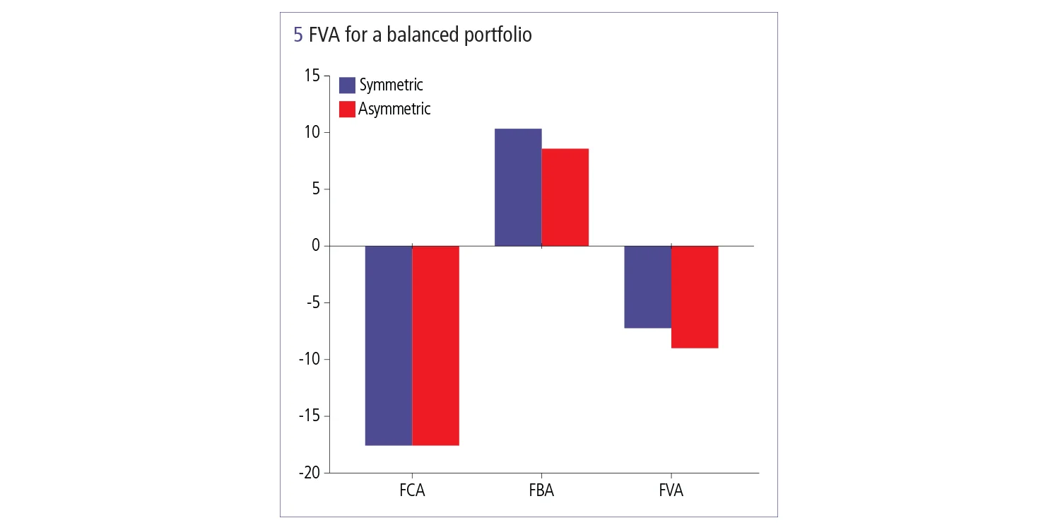
The FBA term is no longer insignificant compared with the FCA term, so the difference in FBA arising from symmetric/asymmetric funding is pronounced and translates into around a 20% difference in FVA.

With the industry likely to adopt asymmetric FVA in the future, banks are faced with a dilemma: do they switch now while they’re asset heavy and take a small writedown or wait until industry adoption is clear but face a large writedown on a more balanced portfolio? 

Parallels could be drawn with the usage of credit spread in the calculation of CVA – whether to use historical or market implied. In this case, banks at the back of the pack took painful losses. It will be interesting to see whether history repeats itself for FVA.

 

^{IHS Markit is a registered trademark of IHS Markit Ltd and/or its affiliates. Opinions, statements, estimates and projections (collectively “information”) in this article are for informational purposes only and are solely those of the individual author(s) at the time of writing and do not necessarily reflect the opinions of IHS Markit. Neither IHS Markit nor the author(s) have any obligations to update this article in the event that any information changes or subsequently becomes inaccurate. IHS Markit makes no warranty, express or implied, as to the accuracy, completeness or timeliness of any information, and shall not in any way be liable to any recipient in respect thereof. ©2019 IHS Markit Ltd. All rights reserved.}

 

XVA – Special report 2019
Read more

Sponsored content