Journal of Risk
ISSN:
1465-1211 (print)
1755-2842 (online)
Editor-in-chief: Farid AitSahlia
Mostly prior-free asset allocation
Sylvain Chassang
Need to know
- The author proposes a novel coherent framework for asset allocation when the past ceases to predict the future.
- The key insight is to replace probability with game theory, and consider the performance of portfolios against an adversarial market.
- The paper shows how to build asset allocation strategies that guarantee low drawdowns against both safe, and risky reference assets.
- The resulting asset allocation strategies improve on classical risk-management strategies such as CPPI or volatility control.
Abstract
This paper develops a prior-free version of Harry Markowitz’s efficient portfolio theory, which allows the decision maker to express their preferences with regard to risk and reward, even though they are unable to express a prior over potentially nonstationary returns. The corresponding optimal allocation strategies are admissible and interior, and they exhibit a form of momentum. Empirically, prior-free efficient allocation strategies successfully exploit the time-varying risk premiums present in historical returns.
Introduction
1 Introduction
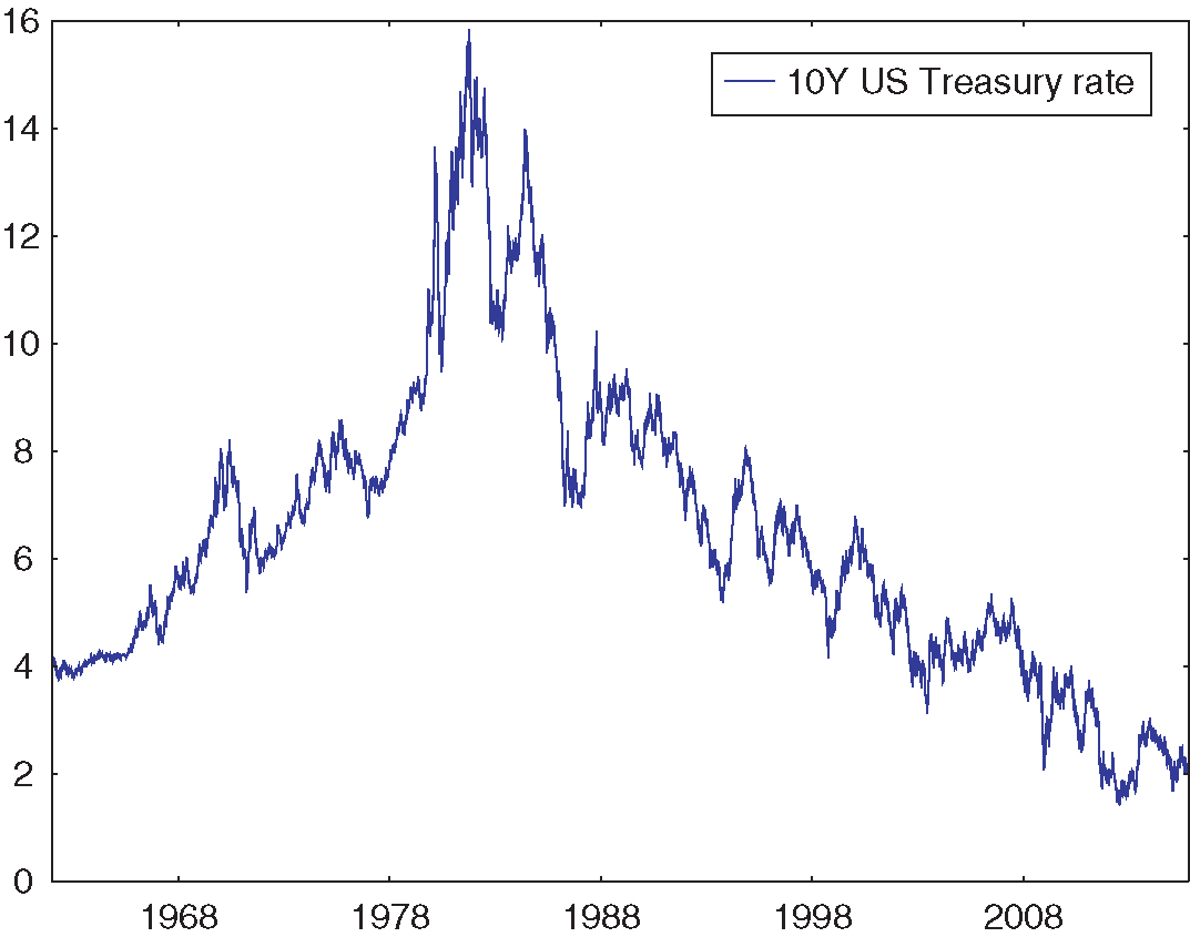
Financial markets are not stationary: they can change in durable ways. Sometimes change is anticipated. For instance, US Treasury yields, which have been going down for the last thirty years, mechanically cannot keep going down much longer (see Figure 1). In this case, we know that the next thirty years must look different. Sometimes, change is only a possibility with which decision makers are concerned. For instance, an investor interested in investing in a smart-beta index fund exploiting one of the familiar premium anomalies (eg, value, momentum, low volatility, low beta) may be plausibly worried that those strategies will become crowded and fail to deliver advertised returns. In a nonstationary environment, past data provides limited guidance on future behavior, which begs the question: how do we make practical risk management and portfolio allocation decisions in such a nonstationary world?

The benchmark framework for portfolio allocation, the efficient portfolio theory of Markowitz (1952), is normatively attractive but requires the decision maker to specify priors over potential returns. This turns out to be practically difficult, even in static settings. Indeed, Black and Litterman (1992) show that when historical data is used to estimate a distribution of returns, plausible implementations of mean–variance optimal portfolios lead to sensitive corner allocations that are intuitively unappealing. In response, they suggest anchoring priors to a neutral prior under which owning a value-weighted portfolio of all assets is optimal. In dynamic environments with a time-varying and possibly nonstationary risk premium, the difficulty of specifying priors is further increased.11See Campbell (1984), Campbell and Viceira (1999) or Lettau and Ludvigson (2001, 2009) for evidence of time variation in risk premiums. The decision maker must specify beliefs over the entire sequence of returns, which is tricky: in high-dimensional state spaces, even full-support priors can exhibit poor frequentist behavior (for instance, failing to converge to true parameters; see, for example, Sims (1971), Diaconis and Freedman (1986) and Ghosh and Ramamoorthi (2003)). As a consequence, neither Markowitz (1952) nor Black and Litterman (1992) provide robust practical frameworks to guide asset allocation in dynamic environments where the process for returns may be nonstationary. Prior-free asset allocation seeks to provide such a framework by giving up on priors all together.
The logic behind prior-free asset allocation matches Harry Markowitz’s description of his actual rather than theoretical approach to portfolio construction (quoted in Zweig (2007)): “I visualized my grief if the stock market went way up and I wasn’t in it – or if it went way down and I was completely in it. My intention was to minimize my future regret. So I split my contributions 50/50 between bonds and equities.” This paper formalizes Markowitz’s intuitive approach as an aversion to worst-case drawdowns (ie, peak-to-trough losses) relative to reference safe and risky assets, in this case, bonds and equities. It solves for the corresponding optimal dynamic asset allocation policy and argues that it provides a systematic framework for asset allocation in nonstationary or novel environments. One simple takeaway is that Markowitz’s 50/50 strategy is optimal in one-shot settings but dominated in dynamic ones.
The model considers an agent who seeks to minimize the worst-case drawdowns of their portfolio relative to benchmark risky and risk-free assets (say the aggregate stock market and short-term US Treasuries). As in other models of non-Bayesian decision making, such as the Gilboa and Schmeidler (1989) model of ambiguity aversion, the framework is game theoretic. Nature is an adversary who seeks to maximize the agent’s drawdowns relative to reference assets. In turn, the agent chooses the dynamic allocation policy that is least gameable by nature. This yields a set of dynamic allocation strategies that achieve minimal worst-case drawdowns relative to all possible sequences of returns. Since these strategies are defined without reference to a prior over returns, this paper refers to these strategies as prior-free optimal.
Our paper makes four points. The first is that prior-free optimal portfolios satisfy a form of robustness to nonstationarity that is not satisfied by more obvious approaches to asset allocation under a time-varying risk premium. Intuitively, asset allocation strategies that experience large drawdowns with respect to either the safe or the risky asset misjudge average geometric returns over a large time window. More generally, large drawdowns can be interpreted as sample violations of optimality conditions. Because a prior-free optimal allocation strategy guarantees small worst-case drawdowns, there is no large time window over which it makes ex-post suboptimal allocation choices. In contrast, any allocation strategy that is Bayesian optimal for a full-support prior over finite hidden Markov models (Baum and Petrie 1966) is gameable by nature: there exists a sequence of returns for which it experiences large drawdowns compared with one of the two reference assets.
The second point is that prior-free asset allocation lets decision makers express preferences with regard to risk and reward in the same way that modern portfolio theory does. Indeed, prior-free optimal strategies define an entire frontier of minimal drawdowns. At one extreme, being fully invested in the market guarantees zero drawdowns against the market at the cost of high worst-case drawdowns against the safe asset. Inversely, being fully invested in the safe asset guarantees zero drawdowns against the safe asset at the cost of high potential drawdowns against the risky asset. The frontier of points in-between lets the decision maker express trade-offs between fear-of-losing (drawdowns against the safe asset) and fear-of-missing-out (drawdowns against the risky asset). Points on this frontier map to dynamic allocation strategies that move smoothly from aggressive to cautious.
The third point is that prior-free optimal strategies are amenable to numerical computation. The agent’s worst-case drawdown minimization problem admits a Bellman representation in which returns are not exogenously drawn from a prior, but rather endogenously picked by nature. The corresponding value function and strategy can be expressed as a function of a four-dimensional summary statistic of past history. This representation allows us to establish some theoretical results of interest: prior-free optimal portfolios are largely interior, and they satisfy a form of momentum. A multi-asset version of the prior-free framework admits an equally tractable representation after appropriate relaxation.
Finally, this paper provides a brief numerical and empirical exploration of this prior-free approach to portfolio optimization. Under worst-case analysis, prior-free portfolios significantly improve on popular portfolio construction rules, such as regularly rebalanced portfolios (RRPs) and constant proportion portfolio insurance (CPPI (Black and Perold 1992)), both of which sit quite far away from the minimal drawdown frontier. More generally, this provides a systematic framework in which to evaluate technical trading rules: any fully specified allocation strategy (this includes RRPs, CPPI, time series momentum, volatility control and moving-average rules) can be mapped against the worst-case drawdown frontier. The benefits of any strategy of interest (eg, the in-sample performance of a volatility-control strategy) can then be weighed against the potential worst-case drawdowns it may experience.
In principle, the high degree of robustness required from prior-free optimal strategies may come at a cost. Indeed, if the true process for returns were independent and identically distributed (iid), a fixed regularly rebalanced portfolio may deliver a better performance than a prior-free optimal portfolio whose allocation changes with realized market returns. This is not the case in the empirical sample of returns. Prior-free optimal strategies perform well in the historical time series of returns, which suggests that they are able to capture time variation in risk premiums present in the data. This is confirmed by a Henriksson and Merton (1981) test. Prior-free portfolios achieve asymmetric exposures to the market in good and bad years (0.7 versus 0.4). Importantly, there is little scope for data-snooping bias (Lo and MacKinlay 1990) when backtesting prior-free optimal strategies. Prior-free optimal portfolios have a single free parameter, the potential magnitude of moves of nature, and this is set in advance of any exposure to data.
The paper connects to an applied literature in portfolio management that seeks to usefully operationalize the approach of Markowitz (1952). Black and Litterman (1992) also place priors at the center of their analysis. They show that naive implementations of Markowitz (1952) are extremely sensitive to prior assumptions over returns or, equivalently, to the sample of data used to calibrate parameters. To address the issue, they suggest anchoring priors to a default prior that rationalizes owning the market portfolio. CPPI, developed in Perold (1986), Black and Jones (1987) and Black and Perold (1992), also avoids priors and proposes a simple class of investment rules that provide risky upside exposure, while providing prior-free downside risk protection. The approach proceeds by using a cushion of safe assets, and leveraging funds above this cushion. However, CPPI can experience large drawdowns with respect to both the safe asset and the risky asset. Grossman and Zhou (1993) tackle the issue of drawdown control in a Bayesian setting, where a fund manager wishes to exploit an asset with known fixed expected returns but is subject to drawdown constraints versus a safe asset.
The worst-case approach emphasized in this paper is related to models of ambiguity aversion axiomatized by Gilboa and Schmeidler (1989) and to multiplier preferences popularized in macroeconomics and finance by Hansen and Sargent (2001, 2008). Cai et al (2000) and Pflug and Wozabal (2007) apply the ambiguity averse framework to static portfolio construction, where it leads to more conservative allocations. Glasserman and Xu (2013, 2014) extend the approach to dynamic environments with trading costs and argue that it leads to a better out-of-sample performance. Note that models based on multiplier preferences still rely on an anchoring prior that nature can perturb at a cost. This theoretical literature has an applied counterpart (see, for example, Ceria and Stubbs 2006; Asl and Etula 2012) that seeks to better take into account model uncertainty when making portfolio allocation decisions.
Because drawdowns use reference assets to benchmark performance, the preferences explored in this paper are related to regret-averse and reference-dependent preferences that have received attention in the statistical (Wald 1950; Savage 1951; Milnor 1954; Stoye 2008) and behavioral literatures (Tversky and Kahneman 1991; Kőszegi and Rabin 2006). It is closely related to the question of online regret minimization originally studied in Blackwell (1956) and Hannan (1957) (for a recent reference, see Cesa-Bianchi and Lugosi (2006)). The portfolio allocation problem studied here is also connected to Cover (1991) and DeMarzo et al (2009), both of which derive prior-free lower bounds on portfolio performance.
More broadly, this paper contributes to a growing agenda in economics that seeks to rethink economic design questions from a prior-free perspective. Segal (2003), Bergemann and Schlag (2008), Hartline and Roughgarden (2008), Madarász and Prat (2016) and Brooks (2014) study auctions, pricing and screening. Chassang (2013), Carroll (2014) and Antic (2014) study incentive provision. The current paper adds to this agenda in two ways. First, it provides a prior-free version of Markowitz (1952), which allows decision makers to express meaningful preferences with regard to risk and reward while allowing for arbitrary nonstationarity in returns. Second, it provides an empirical evaluation of prior-free approaches in a practical context. It shows that the cost of robustness need not be large and that, in fact, prior-free optimization may improve on existing benchmarks in the realized historical sample. In addition, prior-free approaches reduce concerns of data-snooping bias.
This paper is structured as follows. Section 2 defines the framework and the prior-free asset allocation problem. Section 3 quantifies robustness to nonstationarity and shows that it is not achieved by a natural class of Bayesian optimal policies. Section 4 provides a general Bellman characterization of prior-free optimal allocation policies. Section 5 establishes qualitative properties assuming that trading costs are equal to zero. Section 6 extends the framework to multiple assets and reinterprets low drawdowns as sample versions of optimality conditions. Section 7 provides a brief empirical evaluation of prior-free asset allocation strategies. Section 8 concludes. Appendix A (available online) extends the empirical analysis and discusses decision-theoretic foundations, as well as possible Bayesian refinements, of the prior-free approach. Proofs are contained in Appendix B (also available online) unless mentioned otherwise.
2 Framework
2.1 Setup
Returns
An investor with finite horizon allocates resources across two assets: a safe asset with returns at time denoted by , as well as a risky asset – say the market – with returns at time denoted by (see Section 6 for an extension to multiple risky assets). The set of possible returns at time is denoted by and referred to as moves of nature. For simplicity, and anticipating computational implementation, it is assumed that set is finite and satisfies the following minimal richness assumption.
Assumption 2.1.
There exists such that . There exist such that , and . Set contains at least three nondiagonal returns such that .
In computational applications, set will take the form
Let us denote by an upper bound to the magnitude of returns in .
Allocations
The set of possible allocations is compact and convex. An allocation at the beginning of period yields a return , where denotes the usual dot product.
Given returns for period , and invested wealth at , wealth and asset shares at the beginning of period (denoted ) are given by
| (2.1) |
It is possible to reallocate assets at the beginning of each period, but reallocation is costly. Specifically, moving from to costs a proportion of the existing asset base. Denote by the highest trading cost. In numerical applications, trading costs will take the form with (ie, 20 basis points (bps)). Invested wealth after reallocation is .
Allocation strategies
An allocation strategy maps each history of returns to an allocation . We denote by the set of possible allocation strategies.
Taking into account trading costs, the returns associated with allocation strategy in period , denoted by , take the form
| (2.2) |
For a sufficiently large state space , any allocation strategy can be described as an automaton depending on state with transition rule :
| (2.3) | ||||
| (2.4) |
An initial allocation and a sequence of returns induces the sequence of allocations defined by
This paper seeks to formalize the following normative question: what are good dynamic asset allocation strategies for a decision maker who worries that returns may be arbitrarily nonstationary?
2.2 Bayesian optimal asset allocation
A standard model of dynamic asset allocation might take the following form. A decision maker with investment horizon and log utility over final wealth is able to place a prior over possible returns. Their optimal asset allocation strategy then solves
| (2.5) |
Unfortunately, this positive description of behavior provides little normative guidance to investors. This becomes particularly clear after mapping the problem of choosing an asset allocation strategy in the axiomatic framework of subjective utility theory (Savage 1972). A realized sequence of returns is an event. A dynamic asset allocation strategy is a Savage act, mapping events to financial outcomes for the decision maker. Provided that a decision maker has well-behaved preferences over acts, subjective expected utility theory tells us that the decision maker’s behavior can be represented as maximizing an expected utility function.
Subjective utility theory is not a normative framework. Priors are inferred from preferences over acts; optimal acts are not obtained from priors. Still, subjective utility theory is routinely used for normative purposes. Black and Litterman (1992) implicitly highlight some of the difficulties that normative uses of subjective expected utility generate. They specify a Gaussian prior over returns and use historical estimates to set mean and covariance parameters. Presuming mean–variance preferences, they show that such beliefs imply extreme corner allocations that are intuitively unappealing. They then propose using priors that would justify holding a value-weighted portfolio. The ex post assessment of Black and Litterman (1992) that extreme allocations are unappealing, and their response – modifying priors until they yield a more palatable allocation – demonstrate that priors are an output, inferred from preferences over actions, and not a primitive of the decision problem.
The normative decision rule, which would start by eliciting beliefs and then maximizing utility, is even more tricky to implement in the dynamic setting considered in this paper. When the process for returns is potentially nonstationary, picking well-behaved priors turns out to be difficult. The literature on frequentist properties of Bayesian estimates (Diaconis and Freedman 1986; Ghosh and Ramamoorthi 2003) shows that generic priors over large-dimensional objects (here, sequences of returns) may fail to satisfy consistency properties that common frequentist estimators robustly satisfy. Section 3 makes this point concretely.
2.3 Mostly prior-free asset allocation
This paper is written from a normative perspective. It specifies preferences over allocation strategies, argues that they are intuitively appealing and studies the strategies that maximize them. Markowitz’s description of his own investment behavior suggests the following three observations:
- •
decision makers fear net losses;
- •
decision makers fear missing out on potential gains; and
- •
decision makers do not have sophisticated beliefs over patterns of returns.
Definitions 2.2, 2.3 and 2.4 formalize preferences over allocation strategies that capture these premises.
Definition 2.2 (Relative drawdowns).
Given an allocation strategy and a sequence of returns , drawdowns and relative to the safe and risky asset are defined as
| (2.6) | ||||
| (2.7) |
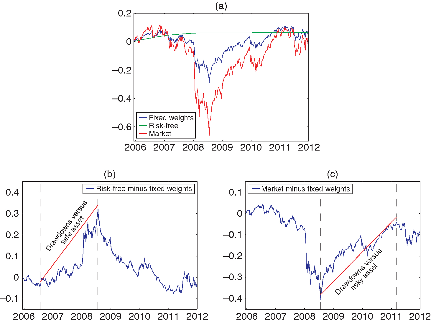
Given realized returns , the relative drawdowns of strategy correspond to strategy ’s maximum relative losses against the safe and risky assets over arbitrary subperiods . Figure 2 shows how to compute the drawdowns of a 50/50 fixed-weight strategy over the market and the risk-free rate during the 2007–12 period.22Returns are obtained from Kenneth French’s data library, available at http://bit.ly/1jwasZk. Note that the time windows over which each drawdown occurs are different for the risk-free and risky assets.

Definition 2.3 (Worst-case drawdowns).
Given a strategy , worst-case drawdowns are defined by
| (2.8) | ||||
| (2.9) |
Potential net losses are captured by strategy ’s worst-case drawdown against the safe asset. Potential foregone gains are captured by strategy ’s worst-case drawdown against the risky asset.
The decision maker’s fear-of-loss and fear-of-missing out are expressed by their willingness to trade off drawdowns against the safe and risky assets. Allocation strategies that attain optimal trade-offs are referred to as prior-free optimal.
Definition 2.4 (Prior-free efficient portfolios).
A portfolio allocation strategy is prior-free efficient if there exists such that solves
Given , denote by a solution to . The corresponding drawdowns are denoted by . The minimal drawdown frontier is described by
Define the associated function .
Lemma 2.5.
Frontier mapping is continuous and strictly decreasing.
Frontier lets the investor make continuous trade-offs between fear-of-loss and fear-of-missing-out in a simple and straightforward manner. Given a tolerable worst case drawdown against the safe asset, it returns the best possible drawdown guarantee against the risky asset.
Two extreme points
Two points of the frontier are easily characterized. At one extreme, it is possible to ensure no drawdowns against the safe asset by being entirely invested in the safe asset. This results in the largest possible drawdowns against the risky asset. Inversely, it is possible to ensure no drawdowns against the risky asset by being entirely invested in the risky asset. This results in the largest possible drawdowns against the safe asset.
The remainder of this paper is interested in the set of points in between these two extremes. It argues that the corresponding prior-free asset allocation strategies achieve the following desiderata: (i) they provide robust performance guarantees for arbitrarily nonstationary processes for returns; (ii) they let the decision maker express meaningful risk preferences over complex acts in a simple manner; and (iii) they perform well in the data.
3 Robustness to nonstationarity
This section motivates the use of prior-free optimal strategies by (i) highlighting their robustness to nonstationarity, and (ii) highlighting the difficulty of finding priors that lead to robust Bayesian-optimal strategies. Section 6 further motivates the use of drawdown-minimizing strategies by reinterpreting drawdowns as sample versions of standard optimality conditions.
3.1 Drawdown control and robustness
Intuitively, strategies that guarantee low drawdowns perform well in environments with time-varying risk premiums, since they guarantee performance close to that of the best-performing asset over any subperiod . This is captured by the following performance bound.
Proposition 3.1 (A performance bound).
Consider a strategy and a sequence of returns . For all time periods , and for all ,
For all time sequences ,
In other words, drawdown guarantees imply lower bounds on the performance of strategy . Up to a penalty , it performs at least as well as asset over any subperiod .
Conversely, a strategy that experiences a large drawdown (say of order ) vis à vis either asset is making a binary allocation error (whether to be invested in the safe or risky asset) over a long period of time. This motivates the following definition.
Definition 3.2.
A sequence of asset allocation strategies (indexed on increasing time horizon ) is said to be robust to nonstationarity if and only if
We now show that for a natural class of full-support priors, Bayesian optimal strategies are not robust to nonstationarity.
3.2 Fragility of finite hidden Markov models
Hidden Markov models are a popular and flexible way to model time-varying processes. However, Proposition 3.3 (below) shows that priors over hidden Markov models lead to strategies that can be defeated by an adversarial nature.
A -state hidden Markov chain over returns with states in is described by , where is a Markov chain describing transitions between unobserved states (with initial state normalized to ), and maps states into distributions over observed returns . A hidden Markov chain induces a stochastic process over unobserved states and observed returns defined by , and
Note that the set of hidden Markov chains with fewer than states is finite dimensional and compact. This implies that one can easily define full-support priors over .
Any Bayesian prior over -state hidden Markov chains is associated with Bayesian optimal policies solving
Such a Bayesian-optimal strategy reflects the investor’s updating over the likelihood of different underlying Markov chains as well as the state these chains may be in. Note that the investor’s posterior belief is itself a Markov chain with infinite (in fact continuous) state space . As a result, it is able to capture many transient patterns of returns, and it is a plausible guess that the corresponding allocation policy could be robust in the sense of Definition 3.2. Proposition 3.3 shows that this is not the case.
Proposition 3.3.
Take as given. For any full-support prior there exists such that, for all and any Bayesian optimal strategy ,
In other words, any Bayesian-optimal allocation policy derived from a full-support prior over finite hidden Markov chains is susceptible to drawdowns of order . As a result, it is not robust to nonstationarity.
3.3 The possibility of robustness
To be useful as a selection criterion, robustness to nonstationarity needs to be nonempty. Proposition 3.4 shows that there exist allocation strategies which guarantee sublinear drawdowns for all possible realized sequences of returns.
Proposition 3.4 (Robustness).
For all and , there exists and a strategy such that
| (3.1) |
Together, Propositions 3.3 and 3.4 establish that it is possible to find strategies that are robust to nonstationarity, but they cannot be obtained by modeling the underlying returns as an unknown finite hidden Markov model.
An immediate corollary of Proposition 3.4 is that prior-free optimal strategies are robust to nonstationarity. Indeed, they achieve the smallest possible drawdowns.
Corollary 3.5.
For any the sequence of prior-free optimal strategies (indexed on time horizon ) is robust to nonstationarity.
It is important to note that robustness to nonstationarity is only an asymptotic property that is achieved by many strategies. In this respect, focusing on prior-free optimal strategies, which achieve exact minimal drawdowns, has several benefits.
- •
It provides the best possible control on drawdowns, optimizing constants, which could matter for empirical evaluations with moderate investment horizon .
- •
- •
It provides a benchmark by which to evaluate the robustness of asset allocation strategies that are attractive for other reasons (eg, in-sample performance).
- •
It provides a systematic framework for optimal dynamic allocation that can incorporate relevant economic features of the problem, such as trading costs or restrictions on the process of returns (bounds on P/E ratios).33See Appendix A (available online) for a discussion of various ways to place restrictions, including probabilistic ones, on the set of possible returns.
4 Computing prior-free optimal strategies
This section shows how to express the problem of computing prior-free optimal asset allocation strategies as a manageable dynamic programming problem. The first step is to identify a convenient state space. Consider an allocation strategy .
For , and , define regrets
| (4.1) |
Regret differs from drawdown in that the endpoint of the period over which underperformance is measured is fixed. In fact, we have that . Lemma 4.1 shows that can be used to compute worst-case drawdowns. It is described by a simple dynamic process.
Lemma 4.1.
For all ,
- (i)
for all ;
- (ii)
for all .
Point (i) implies that to compute drawdown-minimizing strategies, it is sufficient to compute regret-minimizing strategies (this result uses the fact that there exists a return such that ). Point (ii) clarifies why this observation is valuable: regrets at time can be computed as a function of regrets at time and returns at time . In contrast, drawdowns at time depend on drawdowns at time , returns at time and returns in previous periods.
Denote by the vector of regrets, and define state . For any , value function over states is recursively defined as follows:
| (4.2) |
where .
This provides a straightforward way to compute prior-free optimal allocation strategies.
Proposition 4.2 (Bellman formulation).
Let . The following hold.
- (i)
. Drawdown minimizing policy depends only on states and is defined by
- (ii)
The Pareto frontier of worst-case drawdowns is described by
(4.3)
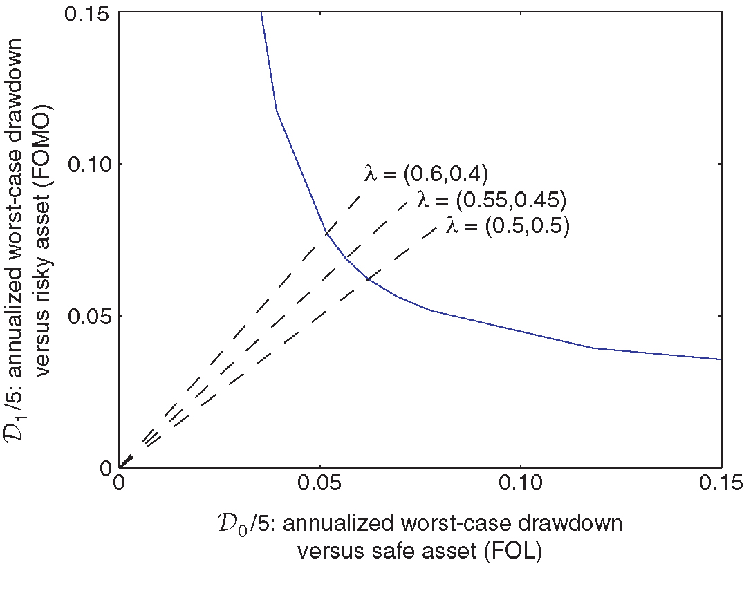
Figure 3 represents the Pareto frontier of minimal drawdowns for moves of nature and time horizon (ie, five years, each period corresponding to a week), computed using the algorithm laid out in Proposition 4.2. Each direction maps to the prior-free optimal allocation strategy such that .
The frontier is convex and sits well to the south-west of the line segment between extreme points corresponding to and . This suggests that it is possible to find attractive trade-offs between fear-of-loss and fear-of-missing-out.

Computing the worst-case drawdowns of arbitrary strategies
This paper focuses on strategies minimizing worst-case drawdowns; however, worst-case drawdowns need not be the only criterion on which allocation strategies are evaluated. In that case, the Pareto frontier characterized by Proposition 4.2 remains useful as a benchmark to evaluate the robustness of alternative strategies that are attractive according to other criteria (eg, in sample performance).
To do this, it is necessary to compute the worst-case drawdowns of arbitrary alternative strategies. Corollary 4.3 (below) shows that the Bellman approach remains useful in this case. Consider an asset allocation strategy defined by an automaton over some state space . For each , define state and introduce the value function over states recursively defined as follows:
| (4.4) |
Corollary 4.3.
For any , let . We have that .
Of course, this Bellman representation is only useful if state space has small dimensionality. When strategy depends on a large state space (which can be the case for strategies depending on truncated moving averages), worst-case drawdowns should be evaluated using Monte Carlo or genetic algorithms approaches designed for high-dimensional numerical optimization (Golberg 1989; Glasserman 2003).
5 Qualitative properties
Proposition 4.2 provides a computational method to characterize drawdown minimizing policies for arbitrary trading costs and arbitrary moves of nature . It is instructive to derive qualitative properties of prior-free optimal allocation strategies under the simplifying assumption that trading costs are equal to 0, and that .
We first note that prior-free optimal strategies are admissible. Recall that denotes the solution to the original maximum–minimum problem .
Proposition 5.1 (Admissibility).
For every , there exists a prior such that
In other words, there always exists a prior over returns for which a prior-free optimal strategy is also Bayesian optimal. Of course, as was emphasized in Sections 2 and 3, the difficulty is coming up with such a prior. The thesis defended by this paper is that expressing preferences over the properties of allocation strategies directly (here, low drawdowns) is consistent with the revealed preference approach, and a practical way to approach dynamic asset allocation.
What prior over moves of nature rationalizes prior-free optimal strategies can be further understood by taking a game-theoretic perspective. Note that, since trading costs are equal to 0, allocation is no longer a state variable. Abusing notation, is now a sufficient state. For any , , , define the payoff function
where .
Lemma 5.2.
- (i)
Payoff function is convex in .
- (ii)
Optimal allocation is a Nash equilibrium strategy in the zero-sum game against nature, with actions and payoffs to the investor.
- (iii)
The drawdown frontier is convex in .
The investor plays a stochastic zero-sum game against nature, and prior-free optimal allocation strategies are Nash equilibriums of this game. This game-theoretic interpretation is helpful in characterizing optimal policies.
5.1 A game-theoretic characterization
Explicit characterization for
Solving for the optimal policy in period helps delineate the mechanics of optimal drawdown control. Note that since returns to the safe asset are equal to 0, nature’s only choice is to pick returns to the risky asset .
At , for regrets , the investor picks the allocation , solving
Lemma 5.3.
- (i)
Whenever , the optimal allocation is strictly interior, ie, .
- (ii)
If , the optimal allocation is . If , the optimal allocation is .
Proof.
Point (ii) is immediate. Whenever , for any allocation and , , which implies that the optimal allocation minimizes , ie, . A similar reasoning holds when .
Point (i) exploits the fact that optimal allocation is a Nash equilibrium in the zero-sum game against nature with payoffs . Hence, it is sufficient to show that neither nor can be part of a Nash equilibrium. Indeed, if , then, since , nature’s strict best response is to set . This yields worst-case regrets , inducing best response from the investor. A similar reasoning shows that cannot be part of an equilibrium either. This implies that the only equilibrium is in mixed strategies. ∎
An immediate corollary is that whenever , . When , since , it is strictly optimal for nature to pick returns in , which implies that . Further, nature must be indifferent to whether or is picked (otherwise, the investor would not use an interior strategy). This implies that an optimal allocation must satisfy
| (5.1) |
This yields the value function
Characterization for
Lemma 5.3 extends as follows. Define and .
Proposition 5.4.
For all , , is continuous in . Further, for all ,
- (i)
if , then ;
- (ii)
if , then , and
(5.2)
5.2 Qualitative implications
Interior allocations
As Black and Litterman (1992) emphasize, naive implementations of the Markowitz (1952) approach to portfolio allocation frequently generate extreme corner allocations. One possible fix is to place ad hoc constraints on allocations. Alternatively, Black and Litterman (1992) suggest anchoring priors to benchmark priors constrained to justify holding the market portfolio. An immediate corollary of Proposition 5.4 is that the prior-free approach naturally leads to noncorner solutions, without the help of ad hoc side constraints.
Corollary 5.5.
For all , there exists such that, for all and all sequences of returns ,
In other words, for any realization of returns, prior-free optimal allocations are interior for a share of periods asymptotically equal to 1.
Momentum
An influential literature documents the profitability of momentum strategies that buy recent overperforming stocks, while selling recent underperforming stocks (Jegadeesh and Titman 1993, 2001; Barberis et al 1998; Hong and Stein 1999; Hong et al 2000; Moskowitz et al 2012; Asness et al 2013), and proposes behavioral explanations for this apparent departure from the efficient market hypothesis.
Even though prior-free optimal strategies are not calibrated using historical data, they, too, exhibit momentum. This reflects the fact that they attempt to optimize asset allocation in arbitrarily nonstationary environments. Returns need not go back to the mean, and momentum emerges as a response to the fact that one asset may well keep performing better than another. Formally, the following result holds.
Corollary 5.6.
Let , with fixed.44As usual, denotes the integer part of , defined as . For any , consider a probability measure over such that, for all ,
Then,
The condition – expected returns weighed by marginal utility are sufficiently high – implies that a history allocating all wealth to the risky asset yields strictly higher expected log returns than any other allocation in .
Corollary 5.6 states that if the returns from the risky asset are drawn from a distribution with sufficiently positive mean over the time interval , then the allocation to the risky asset must go to one. A converse holds if the returns to the risky asset are drawn from a distribution with sufficiently negative mean. Note that to be compatible with Corollary 5.5, Corollary 5.6 requires the allocation to converge to a corner allocation from the interior.
History dependence
Another notable property of prior-free optimal allocation strategies is that even though log preferences do not exhibit a wealth effect, past investment experience affects investors’ continuation behavior. Investors investing in the same period who have experienced different histories of returns will choose different allocations. This is because drawdown minimization is a reference-dependent objective, with the reference point being dependent on an investor’s personal history.
This can be illustrated with a simple example. Consider a two-period investment problem, with time denoted by . A young investor is born in period 1, and an old investor is born in period 0. Both investors share the same preference parameter and the magnitude of potential returns is . Expression (5.1) implies that the young investor will allocate 49.5% of their wealth to the risky asset. The allocation of the old investor depends on their experience at time . We know by Proposition 5.4 that the latter must have chosen an interior allocation in period . If the risky asset yielded returns , they experienced drawdowns against the safe asset, and by (5.1) must place a weight strictly less than on the risky asset. Inversely, if the risky asset yielded returns , they experienced drawdowns against the risky asset, and by (5.1) must place a weight strictly higher than on the risky asset.
This property echoes the finding of Malmendier and Nagel (2011) that investors exhibit heterogeneous risk preferences as a function of their personal histories. Specifically, they show that poor realized returns make investors significantly more risk averse, in a way that is not quantitatively explained by wealth effects.
6 Multi-asset allocation
So far the analysis has focused on allocating resources to a single risky asset. This section extends the prior-free approach to several risky assets. Along the way, it suggests a reinterpretation of drawdowns as optimality conditions.
Framework
Consider an environment with several risky assets and a single risk-free asset denoted by . For simplicity, trading costs are set to zero. Let and , respectively, denote allocations to the risky and risk-free assets at time . Allocations to risky assets must belong to the product set , with . In addition, total allocation weights must sum to , so that . Note that short selling is implicitly allowed. The overall allocation is denoted by . For simplicity, returns to the risk-free asset are constant over time. Risky returns belong to a set of moves of nature taking the form , with . Let .
Consider now the problem of a Bayesian investor maximizing their subjective expected utility. In each period , the investor chooses the allocation that solves
| (6.1) |
where denotes the investor’s information set at . Take as given . For and any allocation , denote by and allocations identical to except that the th coordinate is shifted up or down by an amount . Under the paper’s notation, denotes the weight assigned to asset by allocation . Formally, we have that
By definition, for any , solutions to (6.1) cannot be improved by shifting the allocation in any direction. As a result, for all , under the investor’s prior,
| (6.2) | ||||
| (6.3) |
Using finite sample versions of the central limit theorem, this implies that when returns are drawn from the investor’s prior, then, with probability approaching 1 for large, for all ,55Specifically, the Hoeffding–Azuma inequality. See Cesa-Bianchi and Lugosi (2006), Lemma A.7 for a reference.
| and | ||||
Define drawdowns and as
These drawdowns capture maximal losses relative to strategies that systematically increase or decrease their exposure to a specific asset. Keeping these drawdowns low is a sample expression of the optimality conditions (6.2) and (6.3).
Note that the optimality conditions being tested depend on the step of the deviation . Indeed, the drawdowns studied in Sections 2 to 5 correspond to setting , and . In that case, the drawdowns and of Sections 2–5 satisfy and . Smaller steps , correspond to more local deviations, and potentially allow for finer optimization. For any asset allocation strategy , mapping public histories to allocations, define maximum drawdowns as follows:
Take as given a deviation step , and let be the set of weights such that .66Weights could also be indexed on .
Definition 6.1 (Prior-free allocation strategies).
A dynamic asset allocation strategy is prior-free optimal if there exists such that solves
Computation and key properties
The remainder of this section clarifies difficulties in finding numerical solutions to and identifies an approximately optimal class of strategies amenable to numerical computation and theoretical analysis.
Since there are no trading costs, current allocations are not a state variable in . An argument identical to that of Proposition 4.2 implies that optimal asset allocation policies are a function of state . Unfortunately, the problem of picking an optimal allocation over risk-assets cannot be separated in independent problems. The returns of assets other than affect the optimal allocation to asset . This implies that becomes numerically intractable as the number of risky assets becomes large.
Fortunately, a relaxed problem admits computationally tractable solutions that are approximate solutions to . For any , let
is the set of possible returns differentials due to allocations to assets other than .
Recall the notation and . For all , , , define
For any ,
In , returns are not freely chosen by nature. They are jointly determined by the allocation and returns . The relaxed problem increases nature’s degrees of freedom by allowing it to independently pick and . Denote by and sequences , . For any strategy , mapping histories to the weight assigned to asset , let
Let denote a solution to
This problem is associated with states and the value function
| (6.4) |
Proposition 6.2.
The following hold:
- (i)
for all ;
- (ii)
for all and ;
- (iii)
depends only on states , and solves
In other words, solutions to are easily computable and provide an approximate solution to . The fact that drawdowns are sublinear in implies the following extension of Corollary 5.6.
Let , with fixed. Assume that for returns are iid with a distribution . Further, assume that for all there exists such that
| (6.5) |
where . This implies that problem has a unique corner solution .
Corollary 6.3.
If (6.5) holds, then prior-free optimal strategy satisfies, for all ,
In other words, the prior-free optimal strategy must approach the Bayesian optimal allocation when it takes extreme values. It is worth noting that Corollary 6.3 holds regardless of the history of returns occurring before time . Even after long histories, prior-free optimal allocation strategies do not become doctrinaire. They adapt to new circumstances.
Corollary 6.3 also clarifies that although and let nature pick returns for each asset independently, the resulting strategies respond to correlation between assets. For instance, if one asset is redundant because it is highly correlated to another asset with higher returns, then prior-free asset allocation strategies (relaxed or not) will assign minimal weight to this asset.
7 Practical evaluation
This section evaluates the behavior of prior-free optimal asset allocation against two benchmark risk management strategies (applied to the risk-free asset and a single risky asset):
The solution is implemented as a quarterly rebalanced portfolio, targeting a 50/50 fixed-weight allocation between the safe and risky assets.77Here, the strategy serves as the simplest possible benchmark, similar to a popular 60/40 allocation. The robustness of the approach, as documented by DeMiguel et al (2009), is particularly important when the number of assets becomes large, since in that case the correlation matrix between assets becomes near singular. The current paper makes no empirical claim regarding such many-assets allocation problems. CPPI is an especially relevant benchmark since its goal is to provide prior-free performance guarantees. The version of CPPI tested in this section takes the following form: the investor tracks their counterfactual wealth as if they invested only in the safe asset; a share of their actual wealth equal to 75% of their counterfactual wealth is invested in the safe asset. The remaining cushion is leveraged once and invested in the risky asset. If the price process is continuous and rebalancings occur frequently enough, CPPI guarantees the investor 75% of their wealth if they invested in the safe asset, while also providing exposure to the risky asset.
7.1 Worst-case performance
Figure 4 plots the worst-case drawdowns of both the fixed-weight portfolio and the CPPI portfolio against the prior-free efficient frontier in the case where a period corresponds to a week, , and and the trading cost is equal to 20bps.

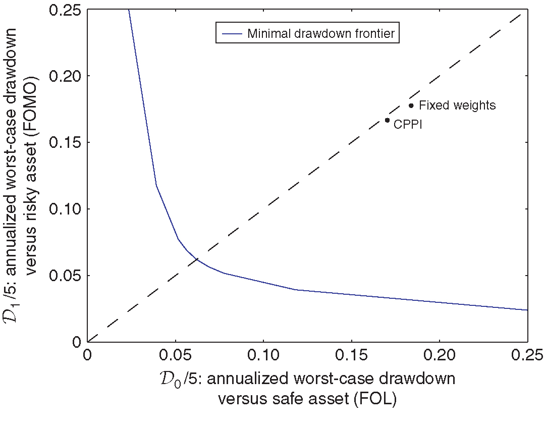
Mechanically, both the fixed-weight portfolio and CPPI must sit to the north-east of the efficient frontier. In fact, they sit quite far away from the efficient frontier.
The reason why the fixed-weight portfolio can experience large drawdowns is clear. It keeps the allocation close to 50/50, even if the risky asset keeps yielding positive (or negative) returns.
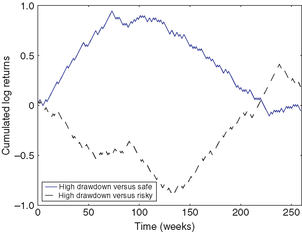
A more surprising finding is that CPPI can also experience large drawdowns, even though it is designed to provide performance guarantees. As Figure 5 illustrates, CPPI experiences drawdowns against the safe asset if the risky asset experiences large gains followed by equally large losses. Indeed, after large gains, CPPI will keep a large exposure to the risky asset until those gains are lost. Inversely, CPPI experiences large drawdowns versus the risky asset if large losses are followed by equally large gains. Indeed, if cumulated losses over a large number of periods make CPPI approach the 75% mark, CPPI will then limit its holding of the risky asset for a commensurate number of periods, resulting in large drawdowns versus the risky asset during the rebound.

7.2 Historical performance
If market returns were iid, prior-free optimal strategies could not possibly improve on the performance of a fixed-weight allocation. However, if risk premiums exhibit significant variation, prior-free optimal strategies may outperform fixed-weight strategies. Whether this is the case is an empirical question.
Table 1 reports findings from running the fixed-weight, CPPI and prior-free optimal strategies defined above on a sample of market and risk-free returns from January 1, 1927 to December 31, 2014, obtained from Kenneth French’s data library. Each strategy is implemented over rolling periods of five years, starting on January 1 for each of the eighty-eight years in the sample. Trading costs are set to 20bps.
Denoting by expectations under the empirical sample of daily returns, the following statistics are reported (counting 252 trading days in a year).
- •
Net annualized performance: .
- •
Annualized Sharpe ratios:
- •
Worst-case five-year relative drawdowns , versus the safe and risky asset over the entire period.
- •
Net performance-to-drawdown ratio:
(7.1) - •
Parameters and from capital asset pricing model regression:
(7.2) estimated using annualized returns (), and reporting robust standard errors.
The net performance-to-drawdown ratio defined in (7.1) summarizes each strategy’s ability to capture upside while reducing drawdowns.
| Fixed | |||
| weights | CPPI | Prior free | |
| Net performance | 3.7% | 4.7% | 6.2% |
| Sharpe | 0.45 | 0.48 | 0.56 |
| 0.54 | 0.37 | 0.29 | |
| 0.44 | 0.53 | 0.37 | |
| Net performance | 0.07 | 0.12 | 0.21 |
| to drawdown | |||
| 0.000 | 0.004 | 0.014 | |
| (0.001) | (0.005) | (0.006) | |
| 0.49 | 0.56 | 0.62 | |
| (0.003) | (0.024) | (0.027) |
The main finding is that instead of reducing in-sample performance, prior-free optimal strategies improve the Sharpe ratio, the performance ratio and especially the performance-to-drawdown ratio of the underlying portfolios. Prior-free asset allocation strategies successfully capture time-varying risk premiums.
Figure 6 reports the cumulative log returns of being long the prior-free portfolio and short the fixed-weight portfolio. The dotted lines separate the sample period into periods of about thirty years: 1927–57, 1957–87 and 1987–2014. The prior-free optimal portfolio overperforms in each subsample, particularly in the 1927–57 sample, where large swings in returns make drawdown control especially valuable. The long–short strategy’s Sharpe ratio over these three subsamples is, respectively, 0.54 (1927–57), 0.20 (1957–87) and 0.30 (1987–2014).

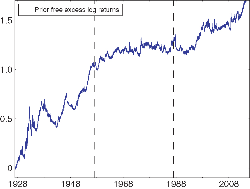
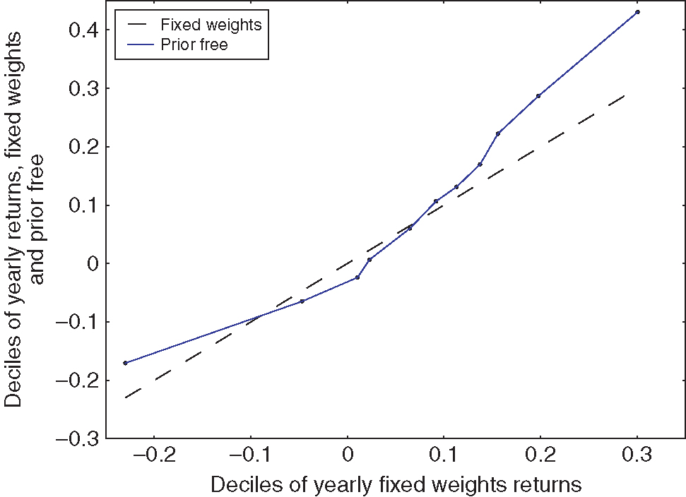
Figure 7 provides further insight into the circumstances in which the prior-free optimal strategy improves on the fixed-weight portfolio. It plots the quantiles of the distribution of returns under the prior-free portfolio against quantiles of the distribution of returns of the fixed-weight portfolio. The prior-free optimal strategy improves both the left and the right tail of returns, but this comes at a cost for yearly returns in the range. This makes intuitive sense: in a range-bound market, the prior-free optimal strategy shifts its allocation following small up and down movements. These adjustments guarantee limited drawdowns in case a bull or bear market should emerge. However, if the market remains range bound, this results in unnecessary transaction costs.

Appendix A (available online) reports further empirical findings. First, a Henriksson and Merton (1981) market-timing regression shows that prior-free optimal asset allocation strategies achieve asymmetric exposure to the market in good and bad years ( versus ). Second, the prior-free allocation strategy improves on a strategy that goes long the market and hedges large losses using put options. Third, the main empirical findings are not sensitive to the choice of parameters used in setting up the drawdown-control problem .
8 Conclusion
This paper provides a prior-free framework for asset allocation in arbitrarily nonstationary environments. The framework allows decision makers to express risk preferences by trading off fear-of-loss (potential drawdowns against the safe asset) and fear-of-missing-out (potential drawdowns against the risky asset). Prior-free optimal allocation strategies are amenable to numerical computation, are largely interior and satisfy a form of momentum. Finally, they are history dependent.
Practically, prior-free optimal strategies offer worst-case drawdown guarantees that are a significant improvement on those offered by fixed-weight strategies or CPPI. In addition, prior-free optimal strategies perform well in the sample of historical returns, showing that the cost of robustness need not be prohibitive. This is encouraging evidence for a growing agenda that seeks to rethink economic design without probabilistically sophisticated decision makers.
Appendix A (available online) presents some extensions. It reports additional information on the behavior of prior-free optimal strategies in data, including robustness checks. In addition, it provides a decision-theoretic perspective on the approach as well as a discussion of how to extend the prior-free framework to include incomplete probabilistic insights, ie, restrictions on the likelihood of aggregate events.
Declaration of interest
The author reports no conflicts of interest. The author alone is responsible for the content and writing of the paper.
Acknowledgements
I am particularly indebted to Markus Brunnermeier and Harrison Hong for guidance and encouragement. This paper benefited from feedback by Yacine Aït-Shalia, Marie Brière, Valentin Haddad, Augustin Landier, Alexey Medvedev, Ulrich Müller, Wolfgang Pesendorfer, Chris Sims, David Sraer, Annette Vissen-Jorgensen and Pablo Winant, as well as seminar participants at Amundi, the Bank of England, Berkeley, Capital Fund Management, Toulouse and Princeton. Alice Wang provided excellent research assistance.
References
- Antic, N. (2014). Contracting with unknown technologies. Unpublished Paper, Princeton University.
- Asl, F. M., and Etula, E. (2012). Advancing strategic asset allocation in a multi-factor world. Journal of Portfolio Management 39, 59–66 (https://doi.org/10.3905/jpm.2012.39.1.059).
- (2013) Asness, C. S., Moskowitz, T. J., and Pedersen, L. H. (2013). Value and momentum everywhere. Journal of Finance 68, 929–985 (https://doi.org/10.1111/jofi.12021).
- (1998) Barberis, N., Shleifer, A., and Vishny, R. (1998). A model of investor sentiment. Journal of Financial Economics 49, 307–343 (https://doi.org/10.1016/S0304-405X(98)00027-0).
- Baum, L. E., and Petrie, T. (1966). Statistical inference for probabilistic functions of finite state Markov chains. Annals of Mathematical Statistics 37, 1554–1563 (https://doi.org/10.1214/aoms/1177699147).
- Bergemann, D., and Schlag, K. H. (2008). Pricing without priors. Journal of the European Economic Association 6, 560–569 (https://doi.org/10.1162/JEEA.2008.6.2-3.560).
- Black, F., and Jones, R. W. (1987). Simplifying portfolio insurance. Journal of Portfolio Management 14, 48–51 (https://doi.org/10.3905/jpm.1987.409131).
- Black, F., and Litterman, R. (1992). Global portfolio optimization. Financial Analysts Journal 48, 28–43 (https://doi.org/10.2469/faj.v48.n5.28).
- Black, F., and Perold, A. (1992). Theory of constant proportion portfolio insurance. Journal of Economic Dynamics and Control 16, 403–426 (https://doi.org/10.1016/0165-1889(92)90043-E).
- Blackwell, D. (1956). An analog of the minimax theorem for vector payoffs. Pacific Journal of Mathematics 6, 1–8 (https://doi.org/10.2140/pjm.1956.6.1).
- Brooks, B. (2014). Surveying and selling: belief and surplus extraction in auctions. Technical Report, Princeton University.
- (2000) Cai, X., Teo, K.-L., Yang, X., and Zhou, X. Y. (2000). Portfolio optimization under a minimax rule. Management Science 46, 957–972 (https://doi.org/10.1287/mnsc.46.7.957.12039).
- Campbell, J. Y. (1984). Asset duration and time varying risk premia. Unpublished Dissertation, Yale University.
- Campbell, J. Y., and Viceira, L. M. (1999). Consumption and portfolio decisions when expected returns are time varying. Quarterly Journal of Economics 114, 433–495 (https://doi.org/10.1162/003355399556043).
- Carroll, G. (2014). Robustness and linear contracts. American Economic Review 105, 536–563 (https://doi.org/10.1257/aer.20131159).
- Ceria, S., and Stubbs, R. A. (2006). Incorporating estimation errors into portfolio selection: robust portfolio construction. Journal of Asset Management 7, 109–127 (https://doi.org/10.1057/palgrave.jam.2240207).
- Cesa-Bianchi, N., and Lugosi, G. (2006). Prediction, Learning, and Games. Cambridge University Press (https://doi.org/10.1017/CBO9780511546921).
- Chassang, S. (2013). Calibrated incentive contracts. Econometrica 81, 1935–1971 (https://doi.org/10.3982/ECTA9987).
- Cover, T. M. (1991). Universal portfolios. Mathematical Finance 1, 1–29 (https://doi.org/10.1111/j.1467-9965.1991.tb00002.x).
- (2009) DeMarzo, P., Kremer, I., and Mansour, Y. (2009). Hannan and Blackwell meet Black and Scholes: approachability and robust option pricing. Technical Report, Stanford University.
- (2009) DeMiguel, V., Garlappi, L., and Uppal, R. (2009). Optimal versus naive diversification: how inefficient is the portfolio strategy? Review of Financial Studies 22, 1915–1953 (https://doi.org/10.1093/rfs/hhm075).
- Diaconis, P., and Freedman, D. (1986). On the consistency of Bayes estimates. Annals of Statistics 14, 1–26 (https://doi.org/10.1214/aos/1176349830).
- Foster, D. P., and Vohra, R. (1999). Regret in the on-line decision problem. Games and Economic Behavior 29, 7–35 (https://doi.org/10.1006/game.1999.0740).
- Ghosh, J. K., and Ramamoorthi, R. (2003). Bayesian Nonparametrics, Volume 1. Springer.
- Gilboa, I., and Schmeidler, D. (1989). Maxmin expected utility with non-unique prior. Journal of Mathematical Economics 18, 141–153 (https://doi.org/10.1016/0304-4068(89)90018-9).
- Glasserman, P. (2003). Monte Carlo Methods in Financial Engineering, Volume 53. Springer Science & Business Media (https://doi.org/10.1007/978-0-387-21617-1).
- Glasserman, P., and Xu, X. (2013). Robust portfolio control with stochastic factor dynamics. Operations Research 61, 874–893 (https://doi.org/10.1287/opre.2013.1180).
- Glasserman, P., and Xu, X. (2014). Robust risk measurement and model risk. Quantitative Finance 14, 29–58 (https://doi.org/10.1080/14697688.2013.822989).
- Golberg, D. E. (1989). Genetic Algorithms in Search, Optimization, and Machine Learning. Addion Wesley.
- Grossman, S. J., and Zhou, Z. (1993). Optimal investment strategies for controlling drawdowns. Mathematical Finance 3, 241–276 (https://doi.org/10.1111/j.1467-9965.1993.tb00044.x).
- Hannan, J. (1957). Approximation to Bayes risk in repeated play. In Contributions to the Theory of Games, Dresher, M., Tucker, A., and Wolfe, P. (eds), Volume 3, pp. 97–139. Princeton University Press.
- Hansen, L. P., and Sargent, T. J. (2001). Robust control and model uncertainty. American Economic Review 91, 60–66 (https://doi.org/10.1257/aer.91.2.60).
- Hansen, L. P., and Sargent, T. J. (2008). Robustness. Princeton University Press (https://doi.org/10.1515/9781400829385).
- Hartline, J. D., and Roughgarden, T. (2008). Optimal mechanism design and money burning. In Symposium on Theory of Computing (STOC), pp. 75–84. ACM Special Interest Group on Algorithms and Computation Theory (https://doi.org/10.1145/1374376.1374390).
- Henriksson, R. D., and Merton, R. C. (1981). On market timing and investment performance II: statistical procedures for evaluating forecasting skills. Journal of Business 54, 513–533 (https://doi.org/10.1086/296144).
- Hong, H., and Stein, J. C. (1999). A unified theory of underreaction, momentum trading, and overreaction in asset markets. Journal of Finance 54, 2143–2184 (https://doi.org/10.1111/0022-1082.00184).
- (2000) Hong, H., Lim, T., and Stein, J. C. (2000). Bad news travels slowly: size, analyst coverage, and the profitability of momentum strategies. Journal of Finance 55, 265–295 (https://doi.org/10.1111/0022-1082.00206).
- Jegadeesh, N., and Titman, S. (1993). Returns to buying winners and selling losers: implications for stock market efficiency. Journal of Finance 48, 65–91 (https://doi.org/10.1111/j.1540-6261.1993.tb04702.x).
- Jegadeesh, N., and Titman, S. (2001). Profitability of momentum strategies: an evaluation of alternative explanations. Journal of Finance 56, 699–720 (https://doi.org/10.1111/0022-1082.00342).
- Kőszegi, B., and Rabin, M. (2006). A model of reference-dependent preferences. Quarterly Journal of Economics 121, 1133–1165 (https://doi.org/10.1093/qje/121.4.1133).
- Lettau, M., and Ludvigson, S. C. (2001). Resurrecting the (C) CAPM: a cross-sectional test when risk premia are time-varying. Journal of Political Economy 109, 1238–1287 (https://doi.org/10.1086/323282).
- Lettau, M., and Ludvigson, S. C. (2009). Measuring and modeling variation in the risk-return trade-off. In The Handbook of Financial Econometrics, Volume 1, Chapter 11, pp. 617–690. Elsevier.
- Lo, A. W., and MacKinlay, A. C. (1990). Data-snooping biases in tests of financial asset pricing models. Review of Financial Studies 3, 431–467 (https://doi.org/10.1093/rfs/3.3.431).
- Lou, D., and Polk, C. (2013). Comomentum: inferring arbitrage activity from return correlations. Working Paper, London School of Economics.
- Luenberger, D. G. (1968). Optimization by Vector Space Methods. Wiley.
- Madarász, K., and Prat, A. (2016). Screening with an approximate type space. Review of Economic Studies 84(2), 790–815.
- Malmendier, U., and Nagel, S. (2011). Depression babies: do macroeconomic experiences affect risk taking? Quarterly Journal of Economics 126, 373–416 (https://doi.org/10.1093/qje/qjq004).
- Markowitz, H. (1952). Portfolio selection. Journal of Finance 7, 77–91.
- Merton, R. C. (1981). On market timing and investment performance I: an equilibrium theory of value for market forecasts. Journal of Business 54, 363–406 (https://doi.org/10.1086/296137).
- Milnor, J. (1954). Games against nature. Working Paper, Rand Corporation.
- (2012) Moskowitz, T. J., Ooi, Y. H., and Pedersen, L. H. (2012). Time series momentum. Journal of Financial Economics 104, 228–250 (https://doi.org/10.1016/j.jfineco.2011.11.003).
- Novy-Marx, R. (2014). Predicting anomaly performance with politics, the weather, global warming, sunspots, and the stars. Journal of Financial Economics 112, 137–146 (https://doi.org/10.1016/j.jfineco.2014.02.002).
- Perold, A. (1986). Constant proportion portfolio insurance. Unpublished Paper, Harvard Business School.
- Pflug, G., and Wozabal, D. (2007). Ambiguity in portfolio selection. Quantitative Finance 7, 435–442 (https://doi.org/10.1080/14697680701455410).
- Savage, L. J. (1951). The theory of statistical decision. Journal of the American Statistical Association 46, 55–67 (https://doi.org/10.1080/01621459.1951.10500768).
- Savage, L. J. (1972). The Foundations of Statistics. Courier Corporation.
- Segal, I. (2003). Optimal pricing mechanisms with unknown demand. American Economic Review 93, 509–529 (https://doi.org/10.1257/000282803322156963).
- Sims, C. A. (1971). Distributed lag estimation when the parameter space is explicitly infinite-dimensional. Annals of Mathematical Statistics 42, 1622–1636 (https://doi.org/10.1214/aoms/1177693161).
- Stein, J. C. (2009). Presidential address: sophisticated investors and market efficiency. Journal of Finance 64, 1517–1548 (https://doi.org/10.1111/j.1540-6261.2009.01472.x).
- Stoye, J. (2008). Axioms for minimax regret choice correspondences. Unpublished Paper, New York University.
- Tversky, A., and Kahneman, D. (1991). Loss aversion in riskless choice: a reference-dependent model. Quarterly Journal of Economics 106, 1039–1061 (https://doi.org/10.2307/2937956).
- Wald, A. (1950). Statistical decision functions. Working Paper, Wiley.
- Zweig, J. (2007). Your Money and Your Brain: How the New Science of Neuroeconomics Can Help Make You Rich. Simon & Schuster.
Only users who have a paid subscription or are part of a corporate subscription are able to print or copy content.
To access these options, along with all other subscription benefits, please contact info@risk.net or view our subscription options here: http://subscriptions.risk.net/subscribe
You are currently unable to print this content. Please contact info@risk.net to find out more.
You are currently unable to copy this content. Please contact info@risk.net to find out more.
Copyright Infopro Digital Limited. All rights reserved.
You may share this content using our article tools. Printing this content is for the sole use of the Authorised User (named subscriber), as outlined in our terms and conditions - https://www.infopro-insight.com/terms-conditions/insight-subscriptions/
If you would like to purchase additional rights please email info@risk.net
Copyright Infopro Digital Limited. All rights reserved.
You may share this content using our article tools. Copying this content is for the sole use of the Authorised User (named subscriber), as outlined in our terms and conditions - https://www.infopro-insight.com/terms-conditions/insight-subscriptions/
If you would like to purchase additional rights please email info@risk.net