Mixing SABR models for negative rates

- Alexandre Antonov, Michael Konikov and Michael Spector
- 07 Apr 2017

Tweet
Facebook
LinkedIn
Save this article
Send to
Print this page

Free stochastic alpha beta rho (SABR), an extension of the SABR model to negative rates, is not guaranteed to be arbitrage free. To resolve this, Alexandre Antonov, Michael Konikov and Michael Spector use an exact formula for the normal free SABR with arbitrary correlation to construct a mixed SABR model, a weighted sum of the normal and free zero-correlation models, that gives closed-form option prices. Added degrees of freedom allow joint to swaptions and constant maturity swap payments

The stochastic alpha beta rho (SABR) process with parameters $(F_{0},v_{0},\beta,\rho,\gamma)$ ¹¹Sometimes $\alpha$ is used instead of $v_{0}$ (see Hagan et al 2002). for a rate $F_{t}$ and its volatility $v_{t}$ follows the stochastic differential equations (SDEs) $\mathrm{d}F_{t}=F_{t}^{\beta}v_{t}\,\mathrm{d}W_{1}$ and $\mathrm{d}v_{t}=\gamma v_{t}\,\mathrm{d}W_{2}$ , with correlation $\mathbb{E}[\mathrm{d}W_{2}\,\mathrm{d}W_{1}]=\rho\,\mathrm{d}t$ and power $0\leq\beta<1$ . The boundary condition at zero is assumed to be absorbing: this enforces positivity and martingality conditions on the rate (see Andreasen & Huge (2013), Antonov et al (2013), Balland & Tran (2013), Hagan et al (2014), Henry-Labordere (2008), Islah (2009), Mercurio & Morini (2009), Paulot (2009) and Rebonato et al (2009) for further references).

When the SABR model was introduced, positivity of the rates seemed certain. In current market conditions, however, where rates are extremely low and even negative, it is important to extend the SABR model to negative rates. For example, figure 1 in Antonov et al (2015a) displays the historical evolution of the Swiss franc interest rates. We see the rates dropping as low as $-2\%$ and ‘sticking’ to zero for certain periods of time, which suggests their probability densities have a singularity at zero.

The simplest way to take negative rates into account is to shift the SABR process to give an SDE of the form $\mathrm{d}F_{t}=(F_{t}+s)^{\beta}v_{t}\,\mathrm{d}W_{1}$ , where $s$ is a deterministic positive shift. This moves the lower bound on $F_{t}$ from $0$ to $-s$ . Usually, the shift is selected manually (eg, to $2\%$ in the case of short rates of the Swiss franc) and we calibrate the standard parameters $(v_{0},\beta,\rho,\gamma)$ to the swaptions and other available information. There is always a danger that the rates will go lower than anticipated, and we will need to change this parameter accordingly. That can result in jumps in the other SABR parameters as the calibration responds to such readjustment. As a consequence, there will be jumps in the values/Greeks of all volatility-dependent trades. Other drawbacks of the shifted SABR model can be found in Antonov et al (2015a).

Antonov et al (2015a) also presented a more elegant solution to permit negative rates: the free SABR model, $\mathrm{d}F_{t}=|F_{t}|^{\beta}v_{t}\,\mathrm{d}W_{1}$ , with $0\leq\beta<\smash{\tfrac{1}{2}}$ and a free boundary. Such a model allows for negative rates and contains a certain ‘stickiness’ at zero. Moreover, the model satisfies norm-preserving and martingale requirements. We derived the exact option price for the zero-correlation case and an accurate approximation for general correlations. However, the approximation accuracy can degenerate in some cases (especially those related to large strikes and high correlation).

In this article, we build on the normal SABR with free boundary, $\mathrm{d}F_{t}=v_{t}\,\mathrm{d}W_{1}$ . The analytical expression for the option value first appeared in Korn & Tang (2013) in the form of a two-dimensional integral. Below, we present an equivalent one-dimensional integral formula, where the integrand can be approximated with high accuracy in closed form. This way, the model becomes feasible for calibration purposes.

We construct a new model as a mixture of the normal SABR and the zero-correlation free SABR. This model is arbitrage free²²We are talking about arbitrage in the sense of basic options strategies, ie, prices implying negative probability density. and exact in its option-pricing analytical formula. Moreover, it contains more parameters to ensure an accurate calibration to swaptions and constant maturity swap (CMS) payments. In the numerical experiments, we demonstrate the superiority of the mixed SABR over the shifted and free SABR models.

In what follows, we consider only the $F_{0}>0$ case, as we handle the $F_{0}<0$ case in the same way as Antonov et al (2015a).

1 Free-boundary SABR

We briefly review the main properties of the free-boundary SABR (or free SABR):

	$\displaystyle\mathrm{d}F_{t}$	$\displaystyle=\|F_{t}\|^{\beta}v_{t}\,\mathrm{d}W_{1}$		(1)
	$\displaystyle\mathrm{d}v_{t}$	$\displaystyle=\gamma v_{t}\,\mathrm{d}W_{2}$		(2)

for $0\leq\beta<\smash{\tfrac{1}{2}}$ . This model permits negative rates, and the underlying rates exhibit ‘stickiness’ at zero (see Antonov et al 2015a).

The zero-correlation free SABR model can be solved exactly. The option time value can be written as:

	$\displaystyle\mathcal{O}_{F}(T,K)$	$\displaystyle=\mathbb{E}[(F_{T}-K)^{+}]-(F_{0}-K)^{+}$
		$\displaystyle=\frac{1}{\pi}\sqrt{\|KF_{0}\|}\{\bm{1}_{K\geq 0}A_{1}+\sin(\|\nu\|% \pi)A_{2}\}$		(3)

with integrals:

	$\displaystyle A_{1}$	$\displaystyle=\int_{0}^{\pi}\mathrm{d}\phi\,\frac{\sin\phi\sin(\|\nu\|\phi)}{b-% \cos\phi}\frac{G(T\gamma^{2},s(\phi))}{\cosh s(\phi)}$
	$\displaystyle A_{2}$	$\displaystyle=\int_{0}^{\infty}\mathrm{d}\psi\,\frac{\sinh\psi(\bm{1}_{K\geq 0% }\cosh(\|\nu\|\psi)+\bm{1}_{K<0}\sinh(\|\nu\|\psi))}{b+\cosh\psi}\frac{G(T\gamma^{% 2},s(\psi))}{\cosh s(\psi)}$

where:

\nu=-\frac{1}{2(1-\beta)}\quad\text{and}\quad b=\frac{|F_{0}|^{2(1-\beta)}+|K|% ^{2(1-\beta)}}{2|F_{0}K|^{1-\beta}}

Here, $s$ is the following function of $\phi$ and $\psi$ , respectively:

	$\displaystyle\sinh s(\phi)$	$\displaystyle=\gamma v_{0}^{-1}\sqrt{2\bar{q}(b-\cos\phi)}$
	$\displaystyle\sinh s(\psi)$	$\displaystyle=\gamma v_{0}^{-1}\sqrt{2\bar{q}(b+\cosh\psi)}$

where:

\bar{q}=\frac{|F_{0}K|^{1-\beta}}{(1-\beta)^{2}}.

The function:

G(t,s)=2\sqrt{2}\frac{\mathrm{e}^{-t/8}}{t\sqrt{2\pi t}}\int_{s}^{\infty}% \mathrm{d}u\,u\mathrm{e}^{-u^{2}/2t}\sqrt{\cosh u-\cosh s}

(4)

was introduced in Antonov et al (2013). It is closely related to the McKean heat kernel on the hyperbolic plane $\smash{H^{2}}$ . It is important to note that, although the function $G(t,s)$ is a one-dimensional integral, it can be efficiently approximated using a closed formula (see Antonov et al 2013).

Let us move on to a general correlation option time value:

\mathcal{O}_{F}(T,K;v_{0},\beta,\rho,\gamma)=\mathbb{E}[(F_{T}-K)^{+}]-(F_{0}-% K)^{+}

(5)

where we have explicitly restored the SABR parameters. There is no closed form for the general case, so we approximate it using the zero-correlation free SABR model (also called the mimicking model):

\mathrm{d}\tilde{F}_{t}=|\tilde{F}|_{t}^{\tilde{\beta}}\tilde{v}_{t}\,\mathrm{% d}\tilde{W}_{1}\quad\text{and}\quad\mathrm{d}\tilde{v}_{t}=\tilde{\gamma}% \tilde{v}_{t}\,\mathrm{d}\tilde{W}_{2}

with $\smash{\mathbb{E}[\mathrm{d}\tilde{W}_{1}\,\mathrm{d}\tilde{W}_{2}]=0}$ and specially calculated coefficients $\smash{\{\tilde{v}_{0},\tilde{\beta},\tilde{\gamma}\}}$ , where $\smash{\tilde{\beta}}$ and $\smash{\tilde{\gamma}}$ are strike independent:

\tilde{\beta}=\beta\quad\text{and}\quad\tilde{\gamma}^{2}=\gamma^{2}-\tfrac{3}% {2}\{\gamma^{2}\rho^{2}+v_{0}\gamma\rho(1-\beta)F_{0}^{\beta-1}\}

$\tilde{v}_{0}$ is more complicated and strike dependent; its expansion can be found in Antonov et al (2015a). The option time value (5) is then approximated as $\mathcal{O}_{F}(T,K;\tilde{v}_{0},\beta,0,\tilde{\gamma})$ using the closed form (3).

The free SABR call price $\mathcal{C}_{F}^{\,\mathrm{SABR}}(T,K)$ is a smooth function of the strike and forward:

	$\displaystyle\mathcal{C}_{F}$	$\displaystyle\underset{K\rightarrow 0}{=}C_{1}+C_{2}K+C_{3}\|K\|^{2(1-\beta)}+\cdots$
	$\displaystyle\mathcal{C}_{F}$	$\displaystyle\underset{F_{0}\rightarrow 0}{=}C_{1}^{\prime}+C_{2}^{\prime}F_{0% }+C_{3}^{\prime}\|F_{0}\|^{2(1-\beta)}+\cdots$

where the constants $C_{i}$ and $C_{i}^{\prime}$ depend on the model parameters (see Antonov et al (2015a) for more details).

The case $\beta=0$ is clearly regular: it corresponds to the normal free SABR. Looking forward, we note that its option price is the analytical function of the strike and forward at zero. Moreover, there exists an exact formula for the normal free SABR model for any correlation.

2 Normal free-boundary SABR

If we consider the case of a normal SABR with free boundary, ie, $\mathrm{d}F_{t}=v_{t}\,\mathrm{d}W_{1}$ , $\mathrm{d}v_{t}=\gamma v_{t}\,\mathrm{d}W_{2}$ , with some correlation $\mathbb{E}[\mathrm{d}W_{2}\,\mathrm{d}W_{1}]=\rho\,\mathrm{d}t$ , it turns out that the call option’s time value has a closed-form solution:

	$\displaystyle\mathcal{O}_{N}(T,K)$	$\displaystyle=\mathbb{E}[(F_{T}-K)^{+}]-(F_{0}-K)^{+}$
		$\displaystyle=\frac{v_{0}}{\gamma\pi}\int_{s_{0}}^{\infty}\frac{G(\gamma^{2}T,% s)}{\sinh s}\sqrt{\sinh^{2}s-(k-\rho\cosh s)^{2}}\,\mathrm{d}s$		(6)

where:

\cosh s_{0}=\frac{-\rho k+\sqrt{k^{2}+1-\rho^{2}}}{1-\rho^{2}}\quad\text{and}% \quad k=\frac{\gamma(K-F_{0})}{v_{0}}+\rho

The proof of this formula and its comparison with Korn & Tang (2013) is given in Antonov et al (2015b). We note that the option pricing formula appeared first in Korn & Tang (2013) as a two-dimensional integral. The formula above is an equivalent one-dimensional integral formula, where the integrand can be approximated with high accuracy in a closed form. This way, the model becomes feasible for calibration purposes.

It is easy to see that the option price is a regular function of spot and strike even when their values are close to zero. All the derivatives with respect to spot and strike are finite (no ‘stickiness’ at zero).

3 Mixed SABR

Instead of mapping a non-zero-correlation SABR into a zero-correlation one, we can define our model as a mixture of a zero-correlation SABR and a normal SABR. Assume the forward rate $F_{t}$ can be written as:

F_{t}=\chi F_{t}^{(1)}+(1-\chi)F^{(2)}_{t}

where (here, we will write $\alpha$ instead of $v_{0}$ ):

•

$\smash{F_{t}^{(1)}}$ follows a zero-correlation free SABR model with parameters ( $\alpha_{1}$ , $\beta_{1}$ , $0$ , $\gamma_{1}$ );
•

$\smash{F_{t}^{(2)}}$ follows a normal free SABR model with parameters ( $\alpha_{2}$ , $0$ , $\rho_{2}$ , $\gamma_{2}$ );
•

$\chi$ is a random variable, taking a value of $1$ with probability $p$ and a value of $0$ with probability $1-p$ , which is independent of both SABR processes.

The option price for the mixed model is thus a weighted sum:

\mathbb{E}[(F_{T}-K)^{+}]=p\mathbb{E}[(F_{T}^{(1)}-K)^{+}]+(1-p)\mathbb{E}[(F_% {T}^{(2)}-K)^{+}]

One motivation for using this model is that both its branches are SABR processes. It is also arbitrage free, allows rates to go negative and has dynamics similar to the free/shifted SABR (see the end of the numerical experiments).

Both component models have closed-form solutions for option values (3) and (6), implying that the mixed model has an analytical solution:³³The normal model component can be written using the zero beta free SABR form, $\mathcal{O}_{N}(T,K;\alpha_{2},\rho_{2},\gamma_{2})=\mathcal{O}_{F}(T,K;\alpha% _{2},0,\rho_{2},\gamma_{2})$ .

\mathcal{O}_{M}(T,K;\alpha_{1},\beta_{1},\gamma_{1};\alpha_{2},\rho_{2},\gamma% _{2})=p\mathcal{O}_{F}(T,K;\alpha_{1},\beta_{1},0,\gamma_{1})+(1-p)\mathcal{O}% _{N}(T,K;\alpha_{2},\rho_{2},\gamma_{2})

(7)

written as three one-dimensional integrals containing the function $G(t,s)$ (4), which can be very efficiently approximated by a closed formula (see Antonov et al 2013), with errors under 1 basis point. This approximation is far superior to others in the SABR ‘business’, eg, the free SABR approximation for general correlations (Antonov et al 2015a) or the original Hagan one for the absorbing SABR (Hagan et al 2002).

In addition, the mixed SABR gives some extra degrees of freedom, which can be used for calibration to either a larger number of swaptions or to swaptions and CMS quotes. We verify the latter in the numerical experiments below.

Regarding the parameter choices for the mixed SABR, it is always useful to keep the same at-the-money volatility for both models. This leads to the following relationship between the initial stochastic volatilities:

\sigma_{0}=\alpha_{1}F_{0}^{\beta_{1}}=\alpha_{2}

(8)

The other parameters can be independent for greater calibration freedom.

A useful parameterisation of the probability as a function of a parameter $s$ is:

p(s)=\frac{\sigma_{0}\beta_{1}\mathrm{e}^{s}}{\sigma_{0}\beta_{1}\mathrm{e}^{s% }+|\gamma_{2}\rho_{2}|}

(9)

which guarantees the mixed SABR model reduces to either zero-correlation or normal SABR when $\rho_{2}=0$ or $\beta_{1}=0$ , respectively.

The probability $p$ can also be used to control the singularity at zero. Fixing it at some small value reduces the singularity arising from the zero-correlation model. We recommend, however, using the parameterisation (9) for calibration, because the singularity is indeed observed in the rate’s time series (see Antonov et al 2015a, figure 1).

3.1 Parameter intuition

Both branches of the model yield the same ATM volatility (because of the constraint (8)), so the mixed SABR will have the same ATM volatility as well.

The zero-correlation model affects the smile skew through its power $\beta_{1}$ , while the normal model works with the smile skew through its correlation. The mixture of these models dictates the above skew behaviours.

The volatility of volatility $\{\gamma_{1},\gamma_{2}\}$ affects both the smile curvature and the edges. Recall that the large strike limit of the implied Black volatility for SABR is $\gamma/(1-\beta)$ (see Antonov et al 2013). Thus, the mixed model, having one more $\gamma$ parameter than the shifted and free SABR models, can decouple the smile curvature and the edges. This feature allows the mixed SABR to calibrate to both swaptions and CMS quotes. The same goal was achieved by the ZABR model (Andreasen & Huge 2013) employing a numerical solution for option prices.

3.2 Reduced parameterisation

There is also a reduced parameterisation with constraints:

\gamma_{2}=\frac{\gamma_{1}}{1-\beta_{1}}\quad\text{and}\quad p=\frac{\sigma_{% 0}\beta_{1}}{\sigma_{0}\beta_{1}+|\gamma_{2}\rho_{2}|}

(10)

The first constraint ensures the same large strike asymptotics for both models. The second corresponds to the probability parameterisation (9) with $s=0$ , allowing us to recover the pure zero-correlation or normal cases and keep the same skew around the ATM strikes. The reduced parameterisation has the same number of parameters (with similar meanings) as the free SABR case.

4 Comparing the shifted, free and mixed SABR models

Next, we compare the shifted, free and mixed SABR models. As already discussed, the shifted SABR has a shift parameter that is not calibrated but is manually selected and can be invalidated if rates go lower than the chosen value. In this situation, a new value of the shift has to be chosen, which will lead to a jump in other parameters as well as the values/Greeks of all volatility-sensitive instruments.

The free and mixed SABR models are free of this shortcoming: their parameters are either calibrated or set without any future incompatibility with the market.

The analytical formulas for the shifted and free SABR models are approximations. In general, their quality is good, but it can deteriorate in some cases, especially in the wings of the distribution. Sometimes, an ad hoc adjustment is necessary. However, the mixed SABR’s analytics are exact and free of such (sometimes painful) adjustments.

All three models can be calibrated to observed swaption quotes. However, the shifted and free SABR models have too few parameters to attempt a joint calibration to swaptions and CMS quotes. Indeed, they lack extra parameters to control the behaviours of the wings. The mixed SABR has more degrees of freedom and is suitable for such a joint calibration. We address these points in the numerical experiments below.

Finally, the free and mixed SABR models have a singularity at zero that corresponds to the ‘stickiness’ of the rate process at zero, which is observed in the historical rates data. If desired, one can attenuate this singularity by decreasing the probability in the mixed SABR.

5 Numerical experiments

We perform a number of numerical experiments in which we compare our SABR models (shifted, free and mixed). The mixed model is used either in the reduced form (10) or in the full one. We note that the ATM volatilities are always linked together (8).

Table A: 1Y4Y swaption calibration input: strike versus implied normal volatility

Strike (%)	Volatility (bp)
$-$ 0.3	056.42
$-$ 0.11	057.08
0.14	064.2
0.39	071.31
0.89	085.55
1.89	114.32

We take real data from July 1, 2015 for the Swiss franc 1Y4Y (ie, the four year rate in one year’s time) swaptions market with a negative forward rate of $-11$ bp. The input is presented in table A in terms of normal implied volatility in pairs of strike and volatility, $\{K_{i},\sigma_{i}\}$ .

The first exercise is to calibrate our models to these swaptions. As shown in Antonov et al (2015b), the calibration accuracy is very good for all models (the largest error is around 1bp).

A more challenging numerical experiment is a joint calibration to swaptions and a CMS payment. This allows us to demonstrate the superiority of the mixed SABR model.

We recall that the CMS convexity adjustment depends on the variance of the rate process, which can be evaluated by the usual static replication formula (Hagan 2003):

\mathbb{V}[F_{T}]\equiv\mathbb{E}[F_{T}^{2}]-F_{0}^{2}=2\int_{-\infty}^{\infty% }\mathrm{d}K\,\mathcal{O}(T,K)

(11)

As usual, $\mathcal{O}(T,K)$ is an option time value.

Table B: Calibration errors for each SABR model (computed as

\text{calibrated~{}volatility}-\text{input~{}volatility}

, expressed in bp)

	Strike	Input CMS volatility (bp)
Model	(%)	50	60	70	80	90	100
Shifted	$-$ 0.3	$-$ 6.38	$-$ 4.61	$-$ 1.35	$-$ 1.55	$-$ 3.02	$-$ 2.06
	$-$ 0.11	$-$ 0.98	$-$ 0.42	$-$ 1.27	$-$ 1.67	$-$ 1.27	$-$ 0.01
	$-$ 0.14	$-$ 0.58	$-$ 0.61	$-$ 0.01	$-$ 1.13	$-$ 2.45	$-$ 2.89
	$-$ 0.39	$-$ 0.56	$-$ 0.59	$-$ 0.33	$-$ 1.56	$-$ 2.44	$-$ 1.79
	$-$ 0.89	$-$ 1.42	$-$ 0.11	$-$ 0.19	$-$ 0.07	$-$ 0.72	$-$ 3.06
	$-$ 1.89	$-$ 5.70	$-$ 3.71	$-$ 0.41	$-$ 3.27	$-$ 7.36	$-$ 12.15
Free	$-$ 0.3	$-$ 7.10	$-$ 4.88	$-$ 2.36	$-$ 1.43	$-$ 4.01	$-$ 6.37
	$-$ 0.11	$-$ 1.50	$-$ 0.10	$-$ 1.70	$-$ 2.94	$-$ 2.86	$-$ 3.56
	$-$ 0.14	$-$ 0.82	$-$ 0.37	$-$ 0.48	$-$ 1.97	$-$ 4.18	$-$ 4.97
	$-$ 0.39	$-$ 0.55	$-$ 0.53	$-$ 0.75	$-$ 0.60	$-$ 2.34	$-$ 2.60
	$-$ 0.89	$-$ 1.02	$-$ 0.10	$-$ 1.15	$-$ 0.05	$-$ 0.78	$-$ 0.36
	$-$ 1.89	$-$ 4.90	$-$ 3.35	$-$ 1.63	$-$ 1.00	$-$ 1.52	$-$ 3.62
Reduced	$-$ 0.3	$-$ 6.63	$-$ 4.45	$-$ 1.51	$-$ 1.61	$-$ 5.13	$-$ 9.23
mixed	$-$ 0.11	$-$ 1.01	$-$ 0.19	$-$ 1.04	$-$ 1.02	$-$ 0.72	$-$ 0.08
	$-$ 0.14	$-$ 0.42	$-$ 0.28	$-$ 0.02	$-$ 1.72	$-$ 3.61	$-$ 6.34
	$-$ 0.39	$-$ 0.31	$-$ 0.32	$-$ 0.16	$-$ 0.62	$-$ 1.12	$-$ 2.34
	$-$ 0.89	$-$ 1.14	$-$ 0.16	$-$ 0.09	$-$ 1.14	$-$ 2.32	$-$ 2.74
	$-$ 1.89	$-$ 5.77	$-$ 3.47	$-$ 0.70	$-$ 1.54	$-$ 4.32	$-$ 6.14
Mixed	$-$ 0.3	$-$ 6.69	$-$ 4.39	$-$ 1.21	$-$ 0.40	$-$ 0.22	$-$ 0.25
	$-$ 0.11	$-$ 0.98	$-$ 0.45	$-$ 0.99	$-$ 0.99	$-$ 0.90	$-$ 1.13
	$-$ 0.14	$-$ 0.36	$-$ 0.37	$-$ 0.31	$-$ 0.70	$-$ 0.79	$-$ 0.56
	$-$ 0.39	$-$ 0.26	$-$ 0.09	$-$ 0.15	$-$ 0.15	$-$ 0.03	$-$ 0.22
	$-$ 0.89	$-$ 1.12	$-$ 0.69	$-$ 0.09	$-$ 0.33	$-$ 0.19	$-$ 0.42
	$-$ 1.89	$-$ 5.81	$-$ 3.21	$-$ 0.61	$-$ 0.10	$-$ 0.03	$-$ 0.57

Unfortunately, CMS quotes are not always available in the market for a given swap rate. In this article, we analyse the ability of the shifted, free and mixed SABR models to reach different CMS prices. We will quote the CMS payment in terms of its normal implied volatility $\sigma_{\mathrm{CMS}}$ , ie:

\mathbb{E}[F_{T}^{2}]-F_{0}^{2}=T\sigma_{\mathrm{CMS}}^{2}

(12)

Let us determine the minimal volatility $\sigma_{\mathrm{CMS}}$ compatible with the input $\smash{\{K_{i},\sigma_{i}\}_{i=1}^{N}}$ from table A. We construct a curve of the implied volatility $\sigma(K)$ , using linear interpolation between the market nodes $\sigma(K_{i})=\sigma_{i}$ . Next, we integrate the right-hand side of (11) from the first quoted strike to the last one, using the Bachelier formula for the option price:

\mathcal{O}(T,K)=\mathcal{O}_{B}(T,K,\sigma)\equiv\mathbb{E}[(F_{0}-K+\sigma% \sqrt{T}Z)^{+}]-(F_{0}-K)^{+}

(13)

where $Z$ is a standard Gaussian variable with zero mean and unit variance. The minimal CMS volatility, found by:

T\tilde{\sigma}_{\mathrm{CMS}}^{2}=2\int_{K_{1}}^{K_{N}}\mathrm{d}K\,\mathcal{% O}_{B}(T,K,\sigma(K))

(14)

with the input data in table A, will be around 60bp, $\tilde{\sigma}_{\mathrm{CMS}}\simeq\text{60bp}$ . Other interpolations, eg, SABR ones, do not change the answer dramatically, so we can state that the CMS payment with volatility smaller than 60bp is incompatible with the swaptions input.

In our experiments, we examine a joint calibration to the set of swaptions and CMS volatilities from 50bp to 100bp. We analyse the results for all models: shifted, free, reduced mixed and full mixed.

We confirm our theoretical result that CMS volatilities smaller than the minimum value of approximately 60bp cannot be reached by the calibration. (The exact calibration solution does not exist.) Moreover, for attainable CMS volatilities, the full mixed model performs best. (The error is less than 1bp.) This difference is due to the rigidity of the volatility curves of the shifted, free and reduced mixed models; meanwhile, the full mixed model has enough degrees of freedom to maintain the calibrated swaption volatilities with almost independent movement of the wings for the CMS volatility calibration.

Table B shows the calibration errors for each model and indicates a clear winner in terms of accuracy: the mixed model.

Figure 1: Calibrated shifted SABR normal implied volatility

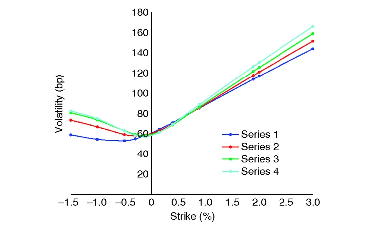
Figure 2: Calibrated free SABR normal implied volatility

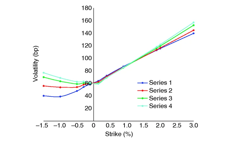
Figure 3: Calibrated reduced mixed SABR normal implied volatility

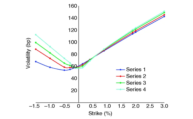
Figure 4: Calibrated mixed SABR normal implied volatility

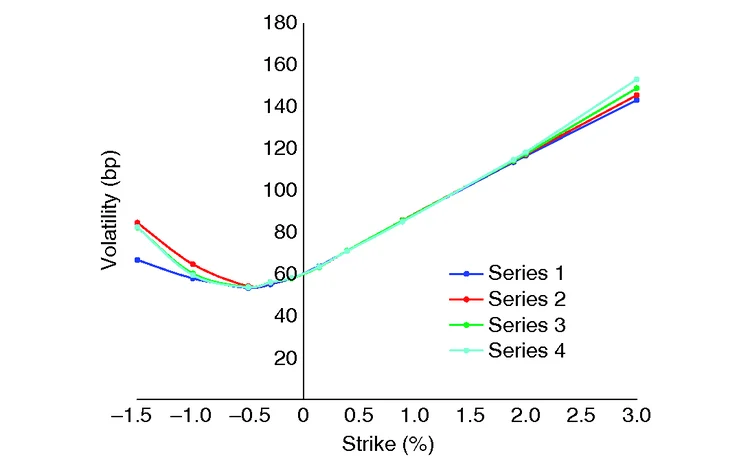
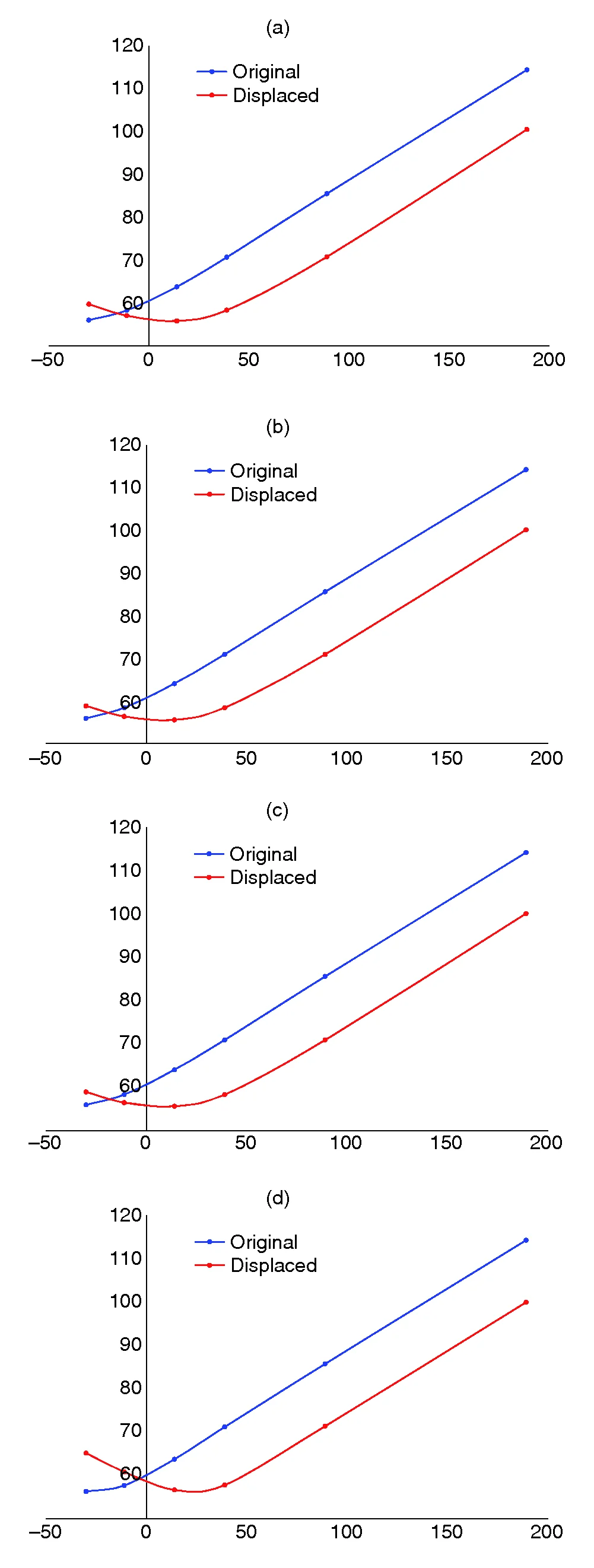
Figure 5: Dynamics of the SABR normal implied volatility (bp) as function of strikes (bp): original forward versus displaced one (a) Shifted. (b) Free. (c) Reduced mixed. (d) Mixed

Table C: 10Y results: all the results are in terms of normal volatilities

Strike (bp)	Exact (bp)	Approx (bp)	Error (bp)
$-$ 506	148.77	148.79	0.01
$-$ 426	141.37	141.38	0.01
$-$ 345	133.82	133.84	0.01
$-$ 264	126.12	126.13	0.01
$-$ 184	118.25	118.26	0.01
$-$ 103	110.19	110.20	0.01
0 $-$ 23	102.01	102.02	0.01
058	096.77	096.78	0.01
139	093.03	093.05	0.01
219	089.89	089.91	0.01
300	087.64	087.65	0.01
381	086.67	086.69	0.01
461	087.48	087.49	0.01
542	090.31	090.32	0.01
623	094.87	094.88	0.01
703	100.62	100.64	0.01
784	107.09	107.11	0.01
864	113.97	113.98	0.01
945	121.07	121.08	0.01
1026	128.29	128.30	0.01
1106	135.55	135.56	0.01

Table D: 10Y mixed SABR parameters

$\alpha_{1}$	$\alpha_{2}$	$\beta$	$\rho$	$\gamma_{1}$	$\gamma_{2}$	$?$
0.0346	0.0085	0.4	$-$ 0.5	0.3	0.3	0.35

In figures 1–4, we present the smiles of our models with the following correspondence of series-CMS volatility:

Series number	1	2	3	4
Input CMS volatility	70	80	90	100

We do not plot the calibrated volatilities for 50bp and 60bp of the CMS volatility, as this is not compatible with the option volatility input. Instead, we concentrate on the larger CMS volatilities and examine how the model does the joint calibration via smile deformation. Figures 1–4 show the calibrated volatilities for each of the SABR models (the underlying explicit numbers can be found in Antonov et al (2015b)).

We observe that only the full mixed model is flexible enough to retain the calibrated option volatilities while adjusting the wings to address the changing CMS volatility. The other models do not have such flexibility, and they deform the option volatilities away from the target.

We now comment on the dynamic properties of the mixed SABR model, ie, the smile behaviour under a displacement of the forward while the other model parameters remain unchanged.⁴⁴In so far as the SABR is mainly the strike interpolator (not a term-structure model), its process-level dynamic properties, ie, conditional expectation $\mathbb{E}[(F_{T}-K)^{+}\mid F_{t}=f]$ , are irrelevant. The SABR’s dynamics was one of the financial motivations for its use (see Hagan et al 2002). In the late 1990s to the early 2000s, the smile moved in the direction of the moving forward. However, it is not a market invariant: now the movement is different. In figure 5, we show the dynamics of the free, shifted and mixed SABRs, with the forward being shifted by 50bp. We see that the results for all three models are similar: the smile follows the rate.

When introducing function $G(t,s)$ in (4), we mentioned that, in practice, we use its one-dimensional approximation as derived in our earlier paper (Antonov et al 2013); a two-dimensional integration would render this model unfeasible. The numbers reported in this paper have been obtained with the approximation of $G(t,s)$ . To show that this does not have much of an effect on the results, we present in table C the normal volatilities for a wide range ( $\pm 3$ standard deviations) of 10-year (10Y) options for a reasonable set of parameters (see table D), with both exact and approximate versions of $G(t,s)$ . As one can see, the differences are well below 1bp.

Figure 6: Implied probability density function of the 10Y swap rate, with exact and approximate G ⁢ ( t , s )

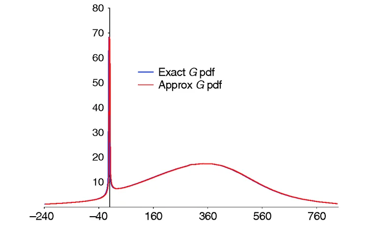
Since our method is based on a one-dimensional integration, and the original Hagan’s formula is written in closed form, our method is about 20–30 times slower. This is consistent with Gaussian quadrature, which requires about 20–30 points for an accurate approximation of an integral. Adaptive quadrature methods, eg, Gauss-Kronrod, may improve the speed of integration in some cases. If the exact function $G(t,s)$ is used, the integration becomes two-dimensional, making it slower than pricing using the approximate $G(t,s)$ by another factor of 20–30. As we do not gain much precision, we recommend always using the approximation. Note that, although when we are theoretically using an approximation of the function $G(t,s)$ we can no longer claim to guarantee the absence of arbitrage, in practice, the quality of our approximation is very good, and we have never encountered any arbitrage (negative probability density) in our tests. Figure 6 shows the implied probability density obtained for the 10Y forward swap rate (with the same parameters as before) using exact and approximate $G(t,s)$ implementations. The plots are practically indistinguishable.

6 Conclusion

In this article, we have presented a new option pricing formula for the normal free SABR model. We have also introduced a new mixed SABR model, which is arbitrage free, allows negative rates and has a closed-form solution for option prices. In addition, the added degrees of freedom allow the mixed SABR model to calibrate to a larger number of swaptions as well as to combinations of swaptions and a single CMS payment.

Alexandre Antonov is a senior vice-president at Numerix in Paris. Michael Konikov is a senior vice-president and the head of quantitative development at Numerix in New York, and Michael Spector is a vice-president at the same firm. The authors are indebted to their colleagues at Numerix, especially Gregory Whitten, Serguei Issakov and Nic Trainor.

Email: antonov@numerix.com,
Email: mkonikov@numerix.com,
Email: mspector@numerix.com.

References

Andreasen J and B Huge, 2013
Expanded forward volatility
Risk January, pages 101–107

Antonov A, M Konikov and M Spector, 2013
SABR spreads its wings
Risk August, pages 58–63

Antonov A, M Konikov and M Spector, 2015a
The free boundary SABR: natural extension to negative rates
Risk September, pages 68–73

Antonov A, M Konikov and M Spector, 2015b
Mixing the SABR for negative rates: analytical arbitrage-free solution
Working Paper, SSRN

Balland P and Q Tran, 2013
SABR goes normal
Risk May, pages 76–81

Hagan P, 2003
Convexity conundrums: pricing CMS swaps, caps, and floors
Wilmott March, pages 38–44

Hagan P, D Kumar, A Lesnievski and D Woodward, 2002
Managing smile risk
Wilmott September, pages 84–108

Hagan P, D Kumar, A Lesnievski and D Woodward, 2014
Arbitrage free SABR
Wilmott January, pages 60–75

Henry-Labordere P, 2008
Analysis, Geometry, and Modeling in Finance: Advanced Methods in Option Pricing
Chapman & Hall

Islah O, 2009
Solving SABR in exact form and unifying it with LIBOR market model
Working Paper, SSRN

Korn R and S Tang, 2013
Exact analytical solution for the normal SABR model
Wilmott July, pages 64–69

Mercurio F and M Morini, 2009
Joining the SABR and Libor models together
Risk March, pages 80–85

Paulot L, 2009
Asymptotic implied volatility at the second order with application to the SABR model
Working Paper, SSRN

Rebonato R, K McKay and R White, 2009
The SABR/LIBOR Market Model: Pricing, Calibration and Hedging for Complex Interest-Rate Derivatives
Wiley

Only users who have a paid subscription or are part of a corporate subscription are able to print or copy content.

To access these options, along with all other subscription benefits, please contact info@risk.net or view our subscription options here: http://subscriptions.risk.net/subscribe

You are currently unable to print this content. Please contact info@risk.net to find out more.

You are currently unable to copy this content. Please contact info@risk.net to find out more.

You may share this content using our article tools. Printing this content is for the sole use of the Authorised User (named subscriber), as outlined in our terms and conditions - https://www.infopro-insight.com/terms-conditions/insight-subscriptions/

If you would like to purchase additional rights please email info@risk.net

You may share this content using our article tools. Copying this content is for the sole use of the Authorised User (named subscriber), as outlined in our terms and conditions - https://www.infopro-insight.com/terms-conditions/insight-subscriptions/

If you would like to purchase additional rights please email info@risk.net